2 Testing the Heckscher-Ohlin Model

The first test of the Heckscher-Ohlin theorem was performed by economist Wassily Leontief in 1953, using data for the United States from 1947. We will describe his test below and show that he reached a surprising conclusion, which is called Leontief’s paradox. After that, we will discuss more recent data for many countries that can be used to test the Heckscher-Ohlin model.

Leontief’s Paradox

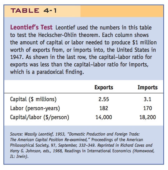
To test the Heckscher-Ohlin theorem, Leontief measured the amounts of labor and capital used in all industries needed to produce $1 million of U.S. exports and to produce $1 million of imports into the United States. His results are shown in Table 4-1.

Leontief first measured the amount of capital and labor required in the production of $1 million worth of U.S. exports. To arrive at these figures, Leontief measured the labor and capital used directly in the production of final good exports in each industry. He also measured the labor and capital used indirectly in the industries that produced the intermediate inputs used in making the exports. From the first row of Table 4-1, we see that $2.55 million worth of capital was used to produce $1 million of exports. This amount of capital seems much too high, until we recognize that what is being measured is the total stock, which exceeds that part of the capital stock that was actually used to produce exports that year: the capital used that year would be measured by the depreciation on this stock. For labor, 182 person-years were used to produce the exports. Taking the ratio of these, we find that each person employed (directly or indirectly) in producing exports was working with $14,000 worth of capital.

Turning to the import side of the calculation, Leontief immediately ran into a problem—he could not measure the amount of labor and capital used to produce imports because he didn’t have data on foreign technologies. To get around this difficulty, Leontief did what many researchers have done since—he simply used the data on U.S. technology to calculate estimated amounts of labor and capital used in imports from abroad. Does this approach invalidate Leontief’s test of the Heckscher-Ohlin model? Not really, because the Heckscher-Ohlin model assumes that technologies are the same across countries, so Leontief is building this assumption into the calculations needed to test the theorem.

Using U.S. technology to measure the labor and capital used directly and indirectly in producing imports, Leontief arrived at the estimates in the last column of Table 4-1: $3.1 million of capital and 170 person-years were used in the production of $1 million worth of U.S. imports, so the capital–labor ratio for imports was $18,200 per worker. Notice that this amount exceeds the capital–labor ratio for exports of $14,000 per worker.

Leontief supposed correctly that in 1947 the United States was abundant in capital relative to the rest of the world. Thus, from the Heckscher-Ohlin theorem, Leontief expected that the United States would export capital-intensive goods and import labor-intensive goods. What Leontief actually found, however, was just the opposite: the capital–labor ratio for U.S. imports was higher than the capital–labor ratio found for U.S. exports! This finding contradicted the Heckscher-Ohlin theorem and came to be called Leontief’s paradox.

Explanations A wide range of explanations has been offered for Leontief’s paradox, including the following:

• U.S. and foreign technologies are not the same, in contrast to what the Heckscher-Ohlin theorem and Leontief assumed.
• By focusing only on labor and capital, Leontief ignored land abundance in the United States.
• Leontief should have distinguished between high-skilled and low-skilled labor (because it would not be surprising to find that U.S. exports are intensive in high-skilled labor).
• The data for 1947 may be unusual because World War II had ended just two years earlier.
• The United States was not engaged in completely free trade, as the Heckscher-Ohlin theorem assumes.

Several of the additional possible explanations for the Leontief paradox depend on having more than two factors of production. The United States is abundant in land, for example, and that might explain why in 1947 it was exporting labor-intensive products: these might have been agricultural products, which use land intensively and, in 1947, might also have used labor intensively. By ignoring land, Leontief was therefore not performing an accurate test of the Heckscher-Ohlin theorem. Alternatively, it might be that the United States was mainly exporting goods that used skilled labor. This is certainly true today, with the United States being a leading exporter of high-technology products, and was probably also true in 1947. By not distinguishing between high-skilled versus low-skilled labor, Leontief was again giving an inaccurate picture of the factors of production used in U.S. trade.

Research in later years aimed to redo the test that Leontief performed, while taking into account land, high-skilled versus low-skilled labor, checking whether the Heckscher-Ohlin theorem holds in other years, and so on. We now discuss the data that can be used to test the Heckscher-Ohlin theorem in a more recent year—2010.

Factor Endowments in 2010

In Figure 4-6, we show the country shares of six factors of production and world GDP in 2010, broken down by select countries (the United States, China, Japan, India, Germany, the United Kingdom, France, and Canada) and then the rest of the world. To determine whether a country is abundant in a certain factor, we compare the country’s share of that factor with its share of world GDP. If its share of a factor exceeds its share of world GDP, then we conclude that the country is abundant in that factor, and if its share in a certain factor is less than its share of world GDP, then we conclude that the country is scarce in that factor. This definition allows us to calculate factor abundance in a setting with as many factors and countries as we want.

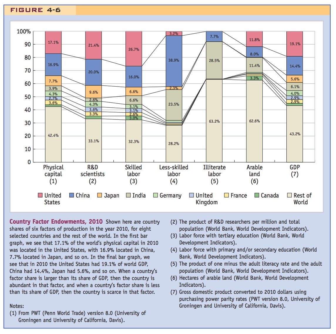
Capital Abundance For example, in the first bar graph of Figure 4-6, we see that in 2010, 17.1% of the world’s physical capital was located in the United States, with 16.9% located in China, 7.7% in Japan, 3.9% in India, 4.3% in Germany, and so on. When we compare these numbers with the final bar in the graph, which shows each country’s percentage of world GDP, we see that in 2010 the United States had 19.1% of world GDP, China had 14.4%, Japan 5.6%, India 6.1%, Germany 4.0%, and so on. Because the United States had 17.1% of the world’s capital and 19.1% of world GDP, we can conclude that the United States was scarce in physical capital in 2010. China, on the other hand, is abundant in physical capital: it has 16.9% of the world’s capital and produces 14.4% of the world’s GDP. Indeed, it is the rapid accumulation of capital in China during the past decade that has now made the United States relatively scarce in this factor (because as China accumulates more capital, the U.S. share of the world’s capital falls).4 Japan had 7.7% of the world’s capital and 5.6% of world GDP in 2010, so it was also abundant in capital, as was Germany (with 4.3% of the world’s capital and 4.0% of world GDP). The opposite holds for India, and the group of countries included in the rest of the world: their shares of world capital were less than their shares of GDP, so they were scarce in capital.

Labor and Land Abundance We can use a similar comparison to determine whether each country is abundant in R&D scientists, in types of labor distinguished by skill, in arable land, or any other factor of production. For example, the United States was abundant in R&D scientists in 2010 (with 21.4% of the world’s total as compared with 19.1% of the world’s GDP) and also skilled labor (workers with more than a high school education) but was scarce in less-skilled labor (workers with a high school education or less) and illiterate labor. India was scarce in R&D scientists (with 2.6% of the world’s total as compared with 6.1% of the world’s GDP) but abundant in skilled labor, semiskilled labor, and illiterate labor (with shares of the world’s total that exceed its GDP share). Canada was abundant in arable land (with 3.3% of the world’s total as compared with 1.7% of the world’s GDP), as we would expect. But the United States was scarce in arable land (11.8% of the world’s total as compared with 19.1% of the world’s GDP). That is a surprising result because we often think of the United States as a major exporter of agricultural commodities, so from the Heckscher-Ohlin theorem, we would expect it to be land-abundant.

Another surprising result in Figure 4-6 is that China was abundant in R&D scientists: it had 20.0% of the world’s R&D scientists, as compared with 14.4% of the world’s GDP in 2010. This finding also seems to contradict the Heckscher-Ohlin theorem, because we think of China as exporting greater quantities of basic manufactured goods, not research-intensive manufactured goods. These observations regarding R&D scientists (a factor in which both the United States and China were abundant) and land (in which the United States was scarce) can cause us to question whether an R&D scientist or an acre of arable land has the same productivity in all countries. If not, then our measures of factor abundance are misleading: if an R&D scientist in the United States is more productive than his or her counterpart in China, then it does not make sense to just compare each country’s share of these with each country’s share of GDP; and likewise, if an acre of arable land is more productive in the United States than in other countries, then we should not compare the share of land in each country with each country’s share of GDP. Instead, we need to make some adjustment for the differing productivities of R&D scientists and land across countries. In other words, we need to abandon the original Heckscher-Ohlin assumption of identical technologies across countries.

Differing Productivities Across Countries

Leontief himself suggested that we should abandon the assumption that technologies are the same across countries and instead allow for differing productivities, as in the Ricardian model. Remember that in the original formulation of the paradox, Leontief had found that the United States was exporting labor-intensive products even though it was capital-abundant at that time. One explanation for this outcome would be that labor is highly productive in the United States and less productive in the rest of the world. If that is the case, then the effective labor force in the United States, the labor force times its productivity (which measures how much output the labor force can produce), is much larger than it appears to be when we just count people. If this is true, perhaps the United States is abundant in skilled labor after all (like R&D scientists), and it should be no surprise that it is exporting labor-intensive products.

We now explore how differing productivities can be introduced into the Heckscher-Ohlin model. In addition to allowing labor to have a differing productivity across countries, we can also allow capital, land, and other factors of production to have differing productivity across countries.

Measuring Factor Abundance Once Again To allow factors of production to differ in their productivities across countries, we define the effective factor endowment as the actual amount of a factor found in a country times its productivity:

The amount of an effective factor found in the world is obtained by adding up the effective factor endowments across all countries. Then to determine whether a country is abundant in a certain factor, we compare the country’s share of that effective factor with its share of world GDP. If its share of an effective factor exceeds its share of world GDP, then we conclude that the country is abundant in that effective factor; if its share of an effective factor is less than its share of world GDP, then we conclude that the country is scarce in that effective factor. We can illustrate this approach to measuring effective factor endowments using two examples: R&D scientists and arable land.

Effective R&D Scientists The productivity of an R&D scientist depends on the laboratory equipment, computers, and other types of material with which he or she has to work. R&D scientists working in different countries will not necessarily have the same productivities because the equipment they have available to them differs. A simple way to measure the equipment they have available is to use a country’s R&D spending per scientist. If a country has more R&D spending per scientist, then its productivity will be higher, but if there is less R&D spending per scientist, then its productivity will be lower. To measure the effective number of R&D scientists in each country, we take the total number of scientists and multiply that by the R&D spending per scientist:

Using the R&D spending per scientist in this way to obtain effective R&D scientists is one method to correct for differences in the productivity of scientists across countries. It is not the only way to make such a correction because there are other measures that could be used for the productivity of scientists (e.g., we could use scientific publications available in a country, or the number of research universities). The advantage of using R&D spending per scientist is that this information is collected annually for many countries, so using this method to obtain a measure of effective R&D scientists means that we can easily compare the share of each country with the world total.5 Those shares are shown in Figure 4-7.

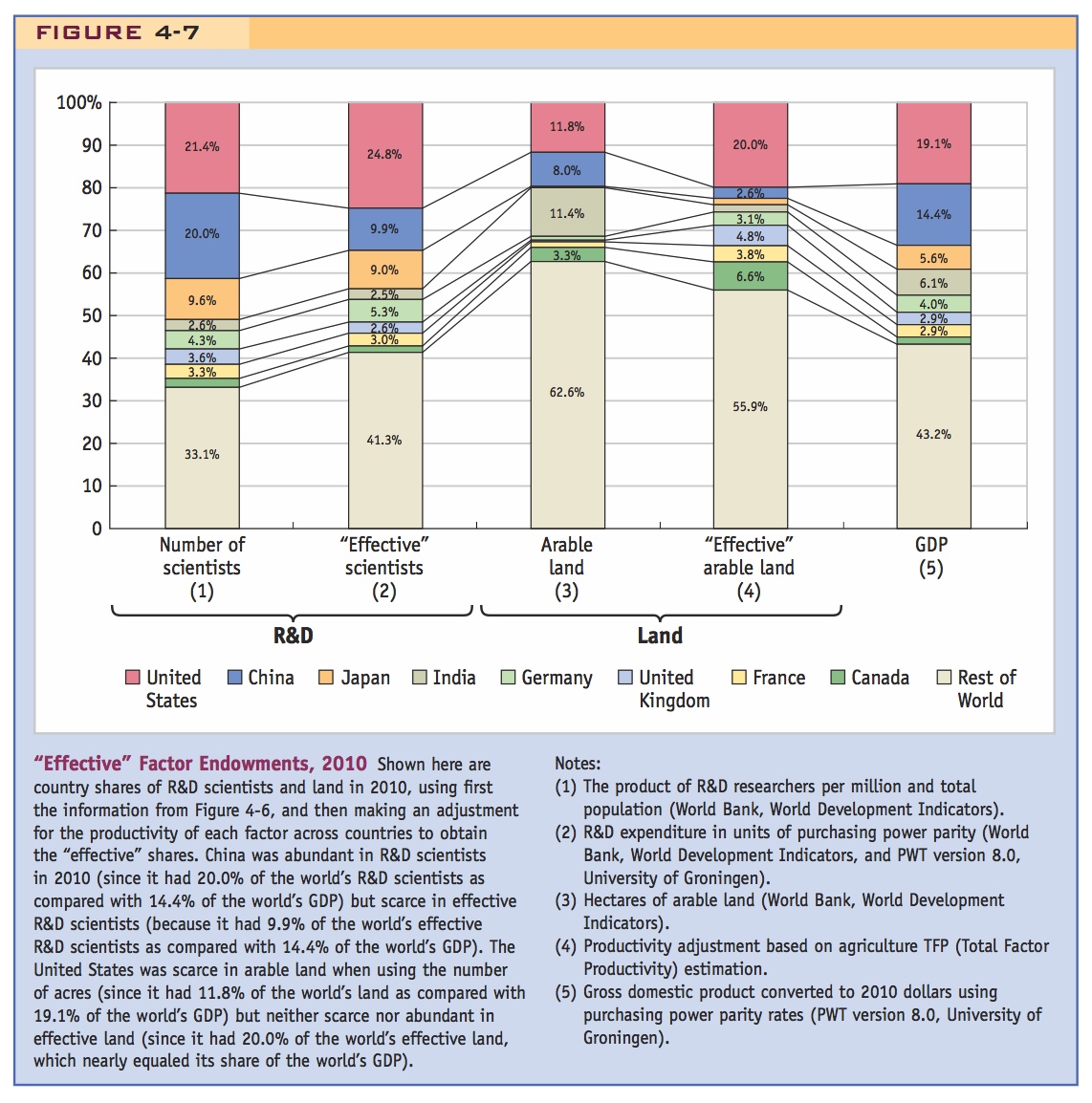
In the first bar graph of Figure 4-7, we repeat from Figure 4-6 each country’s share of world R&D scientists, not corrected for productivity differences. In the second bar graph, we show each country’s share of effective scientists, using the R&D spending per scientist to correct for productivity. The United States had 21.4% of the world’s total R&D scientists in 2010 (in the first bar) but 24.8% of the world’s effective scientists (in the second bar). So the United States was more abundant in effective R&D scientists in 2010 than it was in the number of scientists. Likewise, Germany had a greater share of effective scientists, 5.3%, as compared with its share of R&D scientists, which was 4.3%. But China’s share of R&D scientists fell by half when correcting for productivity, from a 20.0% share in the number of R&D scientists to a 9.9% share in effective R&D scientists. Since China’s share of world GDP was 14.4% in 2010, it became scarce in effective R&D scientists once we made this productivity correction.

China has increased its spending on R&D in recent years and now exceeds the level of R&D spending in Japan. It is also investing heavily in universities, many of which offer degrees in science and engineering. Even when compared with the United States, China is taking the lead in some areas of R&D. An example is in research on “green” technologies, such as wind and solar power. We will discuss government subsidies in China for solar panels in a later chapter. As described in Headlines: China Drawing High-Tech Research from U.S., the Silicon Valley firm Applied Materials has recently established a research laboratory in China and has many contracts to sell solar equipment there. Applied Materials was attracted to China by a combination of inexpensive land and skilled labor. For all these reasons, we should expect that China’s share of effective R&D scientists will grow significantly in future years.

Effective Arable Land As we did for R&D scientists, we also need to correct arable land for its differing productivity across countries. To make this correction, we use a measure of agricultural productivity in each country. Then the effective amount of arable land found in a country is

We will not discuss here the exact method for measuring productivity in agriculture, except to say that it compares the output in each country with the inputs of labor, capital, and land: countries with higher output as compared with inputs are the more productive, and countries with lower output as compared with inputs are the less productive. The United States has very high productivity in agriculture, whereas China has lower productivity.

In the third bar graph of Figure 4-7, we repeat from Figure 4-6 each country’s share of arable land, not corrected for productivity differences. In the fourth bar graph, we show each country’s share of effective arable land in 2010, corrected for productivity differences. The United States had 11.8% of the world’s total arable land (in the third bar), as compared with 19.1% of the world’s GDP (in the final bar), so it was scarce in land in 2010 without making any productivity correction. But when measured by effective arable land, the United States had 20.0% of the world’s total (in the fourth bar), as compared with 19.1% of the world’s GDP (in the final bar). These two numbers are so close that we should conclude the United States was neither abundant nor scarce in effective arable land: its share of the world’s total approximately equaled its share of the world’s GDP.

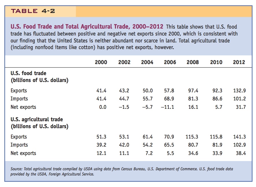
How does this conclusion compare with U.S. trade in agriculture? We often think of the United States as a major exporter of agricultural goods, but this pattern is changing. In Table 4-2, we show the U.S. exports and imports of food products and total agricultural trade. This table shows that U.S. food trade has fluctuated between positive and negative net exports since 2000, which is consistent with our finding that the United States is neither abundant nor scarce in land. Total agricultural trade (including nonfood items like cotton) continues to have positive net exports, however.

Leontief’s Paradox Once Again

Our discussion of factor endowments in 2010 shows that it is possible for countries to be abundant in more that one factor of production: the United States and Japan are both abundant in physical capital and R&D scientists, and the United States is also abundant in skilled labor (see Figure 4-6). We have also found that it is sometimes important to correct that actual amount of a factor of production for its productivity, obtaining the effective factor endowment. Now we can apply these ideas to the United States in 1947 to reexamine the Leontief paradox.

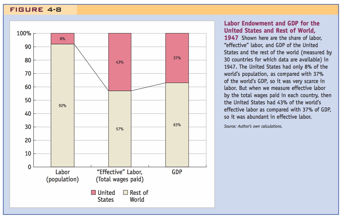
Using a sample of 30 countries for which GDP information is available in 1947, the U.S. share of those countries’ GDP was 37%. That estimate of the U.S. share of “world” GDP is shown in the last bar graph of Figure 4-8. To determine whether the United States was abundant in physical capital or labor, we need to estimate its share of the world endowments of these factors.

Capital Abundance It is hard to estimate the U.S. share of the world capital stock in the postwar years. But given the devastation of the capital stock in Europe and Japan due to World War II, we can presume that the U.S. share of world capital was more than 37%. That estimate (or really a “guesstimate”) means that the U.S. share of world capital exceeds the U.S. share of world GDP, so that the United States was abundant in capital in 1947.

Labor Abundance What about the abundance of labor for the United States? If we do not correct labor for productivity differences across countries, then the population of each country is a rough measure of its labor force. The U.S. share of population for the sample of 30 countries in 1947 was very small, about 8%, which is shown in the first bar graph of Figure 4-8. This estimate of labor abundance is much less than the U.S. share of GDP, 37%. According to that comparison, the United States was scarce in labor (its share of that factor was less than its share of GDP).

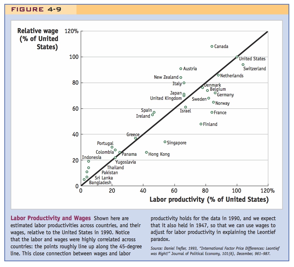
Labor Productivity Using the U.S. share of population is not the right way to measure the U.S. labor endowment, however, because it does not correct for differences in the productivity of labor across countries. A good way to make that correction is to use wages paid to workers as a measure of their productivity. To illustrate why this is a good approach, in Figure 4-9 we plot the wages of workers in various countries and the estimated productivity of workers in 1990. The vertical axis in Figure 4-9 measures wages earned across a sample of 33 countries, measured relative to (i.e., as a percentage of) the United States. Only one country—Canada—has wages higher than those in the United States (probably reflecting greater union pressure in that country). All other countries have lower wages, ranging from Austria and Switzerland with wages that are about 95% of the U.S. wage, to Ireland, France, and Finland, with wages at about 50% of the U.S. level, to Bangladesh and Sri Lanka, with wages at about 5% of the U.S. level.

The horizontal axis in Figure 4-9 measures labor productivity in various countries relative to that in the United States. For example, labor productivity in Canada is 80% of that in the United States; labor productivity in Austria and New Zealand is about 60% of that in the United States; and labor productivity in Indonesia, Thailand, Pakistan, Sri Lanka, and Bangladesh is about 5% of that in the United States. Notice that the labor productivities (on the horizontal axis) and wages (on the vertical axis) are highly correlated across countries: the points in Figure 4-9 line up approximately along the 45-degree line. This close connection between wages and labor productivity holds for the data in 1990 and, we expect that it also held in 1947, so that we can use wages to adjust for labor productivity in explaining the Leontief Paradox.

Effective Labor Abundance As suggested by Figure 4-9, wages across countries are strongly correlated with the productivity of labor. Going back to the data for 1947, which Leontief used, we use the wages earned by labor to measure the productivity of labor in each country. Then the effective amount of labor found in each country equals the actual amount of labor times the wage. Multiplying the amount of labor in each country by average wages, we obtain total wages paid to labor. That information is available for 30 countries in 1947, and we have already found that the United States accounted for 37% of the GDP of these countries, as shown in the final bar in Figure 4-8. Adding up total wages paid to labor across the 30 countries and comparing it with the United States, we find that the United States accounted for 43% of wages paid to labor in these 30 countries, as shown in the bar labeled “effective” labor. By comparing this estimate with the United States share of world GDP of 37% in 1947, we see that the United States was abundant in effective labor, taking into account the differing productivity of labor across countries. So not only was the United States abundant in capital, it was also abundant in effective—or skilled—labor in 1947, just as we have also found for the year 2010!

Summary In Leontief’s test of the Heckscher-Ohlin theorem, he found that the capital–labor ratio for exports from the United States in 1947 was less than the capital–labor ratio for imports. That finding seemed to contradict the Heckscher-Ohlin theorem if we think of the United States as being capital-abundant: in that case, it should be exporting capital-intensive goods (with a high capital–labor ratio). But now we have found that the United States was abundant in both capital and labor in 1947, once we correct for the productivity of labor by using its wage. Basically, the relatively low population and number of workers in the United States are boosted upward by high U.S. wages, making the effective labor force seem much larger—large enough so that the U.S. share of worldwide wages even exceeds its share of GDP.

Such a finding means the United States was also abundant in effective—or skilled—labor in 1947, just as it is today. Armed with this finding, it is not surprising that Leontief found exports from the United States in 1947 used relatively less capital and more labor than did imports: that pattern simply reflects the high productivity of labor in the United States and its abundance of this effective factor. As Leontief himself proposed, once we take into account differences in the productivity of factors across countries, there is no “paradox” after all, at least in the data for 1947. For more recent years, too, taking account of factor productivity differences across countries is important when testing the Heckscher-Ohlin theorem.