3 Effects of Trade on Factor Prices
1. Effect of Trade on the Wage and Rental of Home
a. Economy-Wide Relative Demand for Labor
The economy-wide relative demand curve for labor is a weighted average of the relative demands in the two sectors, where the weights are the shares of capital used in each sector. The relative supply of labor to capital is perfectly inelastic. The equilibrium relative wage (wage/rental) is determined where economy-wide demand and supply are equal.
b. Increase in the Relative Price of Computers
Trade raises the relative price of computers faced by Home. As capital flows into the computer sector, the weights in the economy-wide relative demand shift away from shoes toward computers. The relative demand for labor falls, causing relative wages (W/R) to decrease. The fall in relative wages in turn raises the labor/capital ratio in both sectors.
2. Determination of the Real Wage and Real Rental
What happens to the real wage and rental? Who gains and who loses from trade?
a. Change in the Real Rental
The rental must equal the value of the marginal product in each sector, so that MPKC = R⁄PC and MPKS = R⁄PS. The increase in the labor/capital ratio in both sectors raises the marginal products, so that the real value of the rental, measured in either good, must increase.
b. Change in the Real Wage
Since the labor–capital ratio increases in both sectors, diminishing returns implies that real wages, measured in either good, will fall. That is, both MPLC = W⁄PC and MPLS = W⁄PS both fall. Therefore, the abundant factor gains from trade, while the other factor is hurt.
c. Stolper-Samuelson Theorem
In the long run, when all actors are mobile, an increase in the relative price of a good will increase the real earnings of the factor used intensively in the production of that good and decrease the real earnings of the other factor.
3. Changes in the Real Wage and Rental: A Numerical Example
In the Heckscher-Ohlin model developed in the previous sections, Home exported computers and Foreign exported shoes. Furthermore, we found in our model that the relative price of computers rose at Home from the no-trade equilibrium to the trade equilibrium (this higher relative price with trade is why computers are exported). Conversely, the relative price of computers fell in Foreign from the no-trade equilibrium to the trade equilibrium (this lower relative price with trade is why computers are imported abroad). The question we ask now is how the changes in the relative prices of goods affect the wage paid to labor in each country and the rental earned by capital. We begin by showing how the wage and rental are determined, focusing on Home.
Effect of Trade on the Wage and Rental of Home
To determine the wage and rental, we go back to Figure 4-1, which showed that the quantity of labor demanded relative to the quantity of capital demanded in each industry at Home depends on the relative wage at Home W/R. We can use these relative demands for labor in each industry to derive an economy-wide relative demand for labor, which can then be compared with the economy-wide relative supply of labor  . By comparing the economy-wide relative demand and supply, just as we do in any supply and demand context, we can determine Home’s relative wage. Moreover, we can evaluate what happens to the relative wage when the Home relative price of computers rises after Home starts trading.
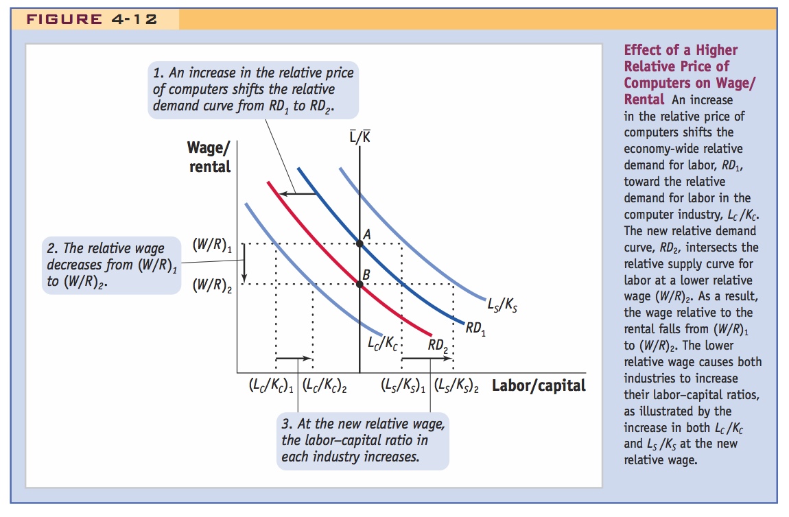
Economy-Wide Relative Demand for Labor To derive an economy-wide relative demand for labor, we use the conditions that the quantities of labor and capital used in each industry add up to the total available labor and capital: LC + LS =  and KC + KS =
  . We can divide total labor by total capital to get
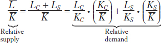
The left-hand side of this equation is the economy-wide supply of labor relative to capital, or relative supply. The right-hand side is the economy-wide demand for labor relative to capital, or relative demand. The relative demand is a weighted average of the labor–capital ratio in each industry. This weighted average is obtained by multiplying the labor–capital ratio for each industry, LC/KC and LS/KS, by the terms KC/ and KS/, the shares of total capital employed in each industry. These two terms must add up to 1, (KC/) + (KS/) = 1, because capital must be employed in one industry or the other.
The determination of Home’s equilibrium relative wage is shown in Figure 4-10 as the intersection of the relative supply and relative demand curves. The supply of labor relative to the supply of capital, the relative supply (), is shown as a vertical line because the total amounts of labor and capital do not depend on the relative wage; they are fixed by the total amount of factor resources in each country. Because the relative demand (the RD curve in the graph) is an average of the LC/KC and LS/KS curves from Figure 4-1, it therefore lies between these two curves. The point at which relative demand intersects relative supply, point A, tells us that the wage relative to the rental is W/R (from the vertical axis). Point A describes an equilibrium in the labor and capital markets and combines these two markets into a single diagram by showing relative supply equal to relative demand.
111
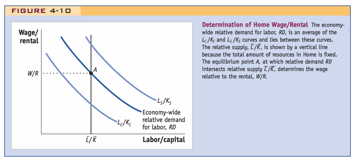
Increase in the Relative Price of Computers When Home opens itself to trade, it faces a higher relative price of computers; that is, PC/PS increases at Home. We illustrate this higher relative price using Home’s production possibilities frontier in Figure 4-11. At the no-trade or autarky equilibrium, point A, the relative price of computers is (PC/PS)A and the computer industry produces QC1, while the shoe industry produces QS1. With a rise in the relative price of computers to (PC/PS)W, the computer industry increases its output to QC2, and the shoe industry decreases its output to QS2. With this shift in production, labor and capital both move from shoe production to computer production. What is the effect of these resource movements on the relative supply and relative demand for labor?
112
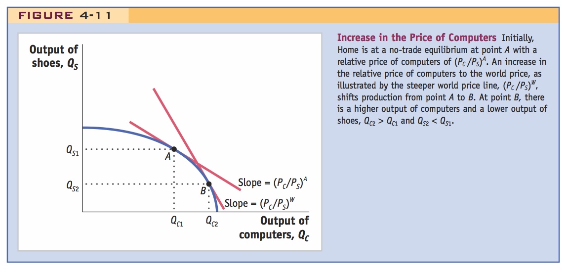
The effects are shown in Figure 4-12. Relative supply is the same as before because the total amounts of labor and capital available in Home have not changed. The relative demand for labor changes, however, because capital has shifted to the computer industry. This shift affects the terms used in the weighted average: (KC/) rises and (KS/) falls. The relative demand for labor in the economy is now more weighted toward computers and less weighted toward the shoe industry. In Figure 4-12, the change in the weights shifts the relative demand curve from RD1 to RD2. The curve shifts in the direction of the relative demand curve for computers, and the equilibrium moves from point A to B.
The impacts on all the variables are as follows. First, the relative wage W/R falls from (W/R)1 to (W/R)2, reflecting the fall in the relative demand for labor as both factors move into computer production from shoe production. Second, the lower relative wage induces both industries to hire more workers per unit of capital (a move down along their relative demand curves). In the shoe industry, for instance, the new, lower relative wage (W/R)2 intersects the relative demand curve for labor LS/KS at a point corresponding to a higher L/K level than the initial relative wage (W/R)1. That is, (LS/KS)2 > (LS/KS)1, and the same argument holds for the computer industry. As a result, the labor–capital ratio rises in both shoes and computers.
113
How is it possible for the labor–capital ratio to rise in both industries when the amount of labor and capital available in total is fixed? The answer is that more labor per unit of capital is released from shoes than is needed to operate that capital in computers (because computers require fewer workers per machine). As the relative price of computers rises, computer output rises while shoe output falls, and labor is “freed up” to be used more in both industries. In terms of our earlier equation for relative supply and relative demand, the changes in response to the increase in the relative price of computers PC/PS are
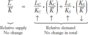
The relative supply of labor has not changed, so relative demand for labor cannot change overall. Since some of the individual components of relative demand have increased, other components must decrease to keep the overall relative demand the same. After the rise in the price of computers, even more capital will be used in the computer industry (KC/ rises while KS/ falls) because the output of computers rises and the output of shoes falls. This shift in weights on the right-hand side pulls down the overall relative demand for labor (this is necessarily true since LC/KC < LS/KS by assumption). But because the relative supply on the left-hand side doesn’t change, another feature must increase the relative demand for labor: this feature is the increased labor–capital ratios in both industries. In this way, relative demand continues to equal relative supply at point B, and at the same time, the labor–capital ratios have risen in both industries.
Determination of the Real Wage and Real Rental
With a little hand-waving, this graphical analysis could be adapted to develop the factor-price equalization theorem.
To summarize, we have found that an increase in the relative price of computers—which are capital-intensive—leads to a fall in the relative wage (W/R). In turn, the decrease in the relative wage leads to an increase in the labor–capital ratio used in each industry (LC/KC and LS/KS). Our goal in this section is to determine who gains and who loses from these changes. For this purpose, it is not enough to know how the relative wage changes; instead, we want to determine the change in the real wage and real rental; that is, the change in the quantity of shoes and computers that each factor of production can purchase. With the results we have already obtained, it will be fairly easy to determine the change in the real wage and real rental.
Change in the Real Rental Because the labor–capital ratio increases in both industries, the marginal product of capital also increases in both industries. This is because there are more people to work with each piece of capital. This result follows from our earlier argument that when a machine has more labor to work it, it will be more productive, and the marginal product of capital will go up. In both industries, the rental on capital is determined by its marginal product and by the prices of the goods:
114
R = PC · MPKC and R = PS · MPKS
Because capital can move freely between industries in the long run, the rental on capital is equalized across them. By using the result that both marginal products of capital increase and by rearranging the previous equations, we see that
MPKC = R/PC ↑ and MPKS = R/PS ↑
Remember that R/PC measures that quantity of computers that can be purchased with the rental, whereas R/PS measures the quantity of shoes that can be bought with the rental. When both of these go up, the real rental on capital (in terms of either good) increases. Therefore, capital owners are clearly better off when the relative price of computers increases. Notice that computer manufacturing is the capital-intensive industry, so the more general result is that an increase in the relative price of a good will benefit the factor of production used intensively in producing that good.
Change in the Real Wage To understand what happens to the real wage when the relative price of computers rises, we again use the result that the labor–capital ratio increases in both industries. The law of diminishing returns tells us that the marginal product of labor must fall in both industries (since there are more workers on each machine). In both industries, the wage is determined by the marginal product of labor and the prices of the goods:
W = PC · MPLC and W = PS · MPLS
Using the result that the marginal product of labor falls in both industries, we see that
MPLC = W/PC ↓ and MPLS = W/PS ↓
Therefore, the quantity of computers that can be purchased with the wage (W/PC) and the quantity of shoes that can be purchased with the wage (W/PS) both fall. These decreases mean that the real wage (in terms of either good) is reduced, and labor is clearly worse off because of the increase in the relative price of computers.
We can summarize our results with the following theorem, first derived by economists Wolfgang Stolper and Paul Samuelson.
Stolper-Samuelson Theorem: In the long run, when all factors are mobile, an increase in the relative price of a good will increase the real earnings of the factor used intensively in the production of that good and decrease the real earnings of the other factor.
Emphasize that S-S is the only fully articulated general equilibrium model of the income distribution that we have.
For our example, the Stolper-Samuelson theorem predicts that when Home opens to trade and faces a higher relative price of computers, the real rental on capital in Home rises and the real wage in Home falls. In Foreign, the changes in real factor prices are just the reverse. When Foreign opens to trade and faces a lower relative price of computers, the real rental falls and the real wage rises. Remember that Foreign is abundant in labor, so our finding that labor is better off there, but worse off at Home, means that workers in the labor-abundant country gain from trade but workers in the capital-abundant country lose. In addition, capital in the capital-abundant country (Home) gains, and capital in the labor-abundant country loses. These results are sometimes summarized by saying that in the Heckscher-Ohlin model, the abundant factor gains from trade, and the scarce factor loses from trade.6
115
Changes in the Real Wage and Rental: A Numerical Example
As in S-F, break the class into groups. Let them create and solve their own numerical examples.
To illustrate the Stolper-Samuelson theorem, we use a numerical example to show how much the real wage and rental can change in response to a change in price. Suppose that the computer and shoe industries have the following data:
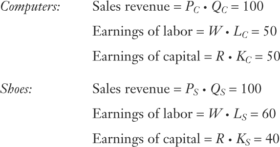
Notice that shoes are more labor-intensive than computers: the share of total revenue paid to labor in shoes (60/100 = 60%) is more than that share in computers (50/100 = 50%).
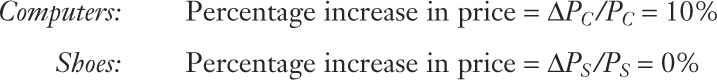
When Home and Foreign undertake trade, the relative price of computers rises. For simplicity we assume that this occurs because the price of computers PC rises, while the price of shoes PS does not change:
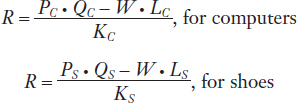
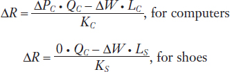
Our goal is to see how the increase in the relative price of computers translates into long-run changes in the wage W paid to labor and the rental on capital R. Remember that the rental on capital can be calculated by taking total sales revenue in each industry, subtracting the payments to labor, and dividing by the amount of capital. This calculation gives us the following formulas for the rental in each industry:7
The price of computers has risen, so Δ PC > 0, holding fixed the price of shoes, Δ PS = 0. We can trace through how this affects the rental by changing PC and W in the previous two equations:
116
It is convenient to work with percentage changes in the variables. For computers, ΔPC/PC is the percentage change in price. Similarly, ΔW/W is the percentage change in the wage, and ΔR/R is the percentage change in the rental of capital. We can introduce these terms into the preceding formulas by rewriting them as
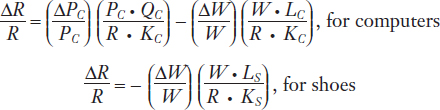
(You should cancel terms in these equations to check that they are the same as before.)
Now we’ll plug the above data for shoes and computers into these formulas:
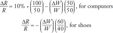
Our goal is to find out by how much rental and wage change given changes in the relative price of the final goods, so we are trying to solve for two unknowns (ΔR/R and ΔW/W) from the two equations given here. A good way to do this is to reduce the two equations with two unknowns into a single equation with one unknown. This can be done by subtracting one equation from the other, as follows:
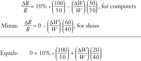
Simplifying the last line, we get 0 = 20% +  , so that
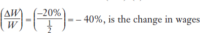
So when the price of computers increases by 10%, the wage falls by 40%. With the wage falling, labor can no longer afford to buy as many computers (W/PC has fallen since W is falling and PC has increased) or as many pairs of shoes (W/PS has fallen since W is falling and PS has not changed). In other words, the real wage measured in terms of either good has fallen, so labor is clearly worse off.
To find the change in the rental paid to capital (ΔR/R), we can take our solution for ΔW/W = − 40%, and plug it into the equation for the change in the rental in the shoes sector:8
117
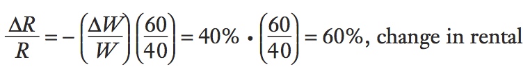
The rental on capital increases by 60% when the price of computers rises by 10%, so the rental increases even more (in percentage terms) than the price. Because the rental increases by more than the price of computers in percentage terms, it follows that (R/PC) rises: owners of capital can afford to buy more computers, even though their price has gone up. In addition, they can afford to buy more shoes (R/PS also rises, since R rises and PS is constant). Thus, the real rental measured in terms of either good has gone up, and capital owners are clearly better off.
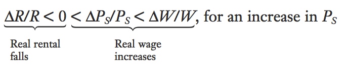
General Equation for the Long-Run Change in Factor Prices The long-run results of a change in factor prices can be summarized in the following equation:
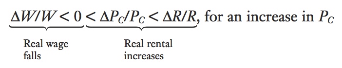
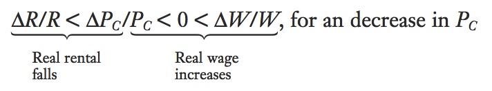
That is, the increase in the price of computers (10%) leads to an even larger increase in the rental on capital (60%) and a decrease in the wage (−40%). If, instead, the price of computers falls, then these inequalities are reversed, and we get
What happens if the relative price of shoes increases? From the Stolper-Samuelson theorem, we know that this change will benefit labor, which is used intensively in shoe production, and will harm capital. The equation summarizing the changes in factor earnings when the price of shoes increases is
These equations relating the changes in product prices to changes in factor prices are sometimes called the “magnification effect” because they show how changes in the prices of goods have magnified effects on the earnings of factors: even a modest fluctuation in the relative prices of goods on world markets can lead to exaggerated changes in the long-run earnings of both factors. This result tells us that some groups—those employed intensively in export industries—can be expected to support opening an economy to trade because an increase in export prices increases their real earnings. But other groups—those employed intensively in import industries—can be expected to oppose free trade because the decrease in import prices decreases their real earnings. The following application examines the opinions that different factors of production have taken toward free trade.
Specific-factor theory predicts workers in export industries should favor free trade; HO predicts that skilled workers in the U.S. should favor free trade, regardless of the industry. Survey supports HO.
Opinions Toward Free Trade
Countries sometimes conduct a survey about their citizens’ attitudes toward free trade. A survey conducted in the United States by the National Elections Studies (NES) in 1992 included the following question:
118
Some people have suggested placing new limits on foreign imports in order to protect American jobs. Others say that such limits would raise consumer prices and hurt American exports. Do you favor or oppose placing limits on imports, or haven’t you thought much about this?
Respondents to the survey could either answer that they “favor” placing limits on imports, meaning that they do not support free trade, or that they “oppose” limits on imports, meaning that they support free trade. How do these answers compare with characteristics of the respondents, such as their wages, skills, or the industries in which they work?
According to the specific-factors model, in the short run we do not know whether labor will gain or lose from free trade, but we do know that the specific factor in the export sector gains, and the specific factor in the import sector loses. Think about an extension of this model, in which, in addition to their wage, labor also earns some part of the rental on the specific factor in their industry. This assumption is true for farmers, for example, who work in agriculture and may own their land; it can also be true for workers in manufacturing if their salary includes a bonus that is based on the profits earned by capital. In those situations, we would expect that workers in export industries will support free trade (since the specific factor in that industry gains), but workers in import-competing industries will be against free trade (since the specific factor in that industry loses). In the short run, then, the industry of employment of workers will affect their attitudes toward free trade.
In the long-run Heckscher-Ohlin (HO) model, however, the industry of employment should not matter. According to the Stolper-Samuelson theorem, an increase in the relative price of exports will benefit the factor of production used intensively in exports and harm the other factor, regardless of the industry in which these factors of production actually work (remember that each factor of production earns the same wage or rental across industries in the long run). In the United States, export industries tend to use high-skilled labor intensively for research and development and other scientific work. An increase in the relative price of exports will benefit high-skilled labor in the long run, regardless of whether these workers are employed in export-oriented industries or import-competing industries. Conversely, an increase in the relative price of exports will harm low-skilled labor, regardless of where these workers are employed. In the long run, then, the skill level of workers should determine their attitudes toward free trade.
In the 1992 NES survey, the industry of employment was somewhat important in explaining the respondents’ attitudes toward free trade, but their skill level was much more important.9 That is, workers in export-oriented industries are somewhat more likely to favor free trade, with those in import-competing industries favoring import restrictions, but this statistical relationship is not strong. A much more important determinant of the attitudes toward free trade is the skill level of workers, as measured by their wages or their years of education. Workers with lower wages or fewer years of education are more likely to favor import restrictions, whereas those with higher wages and more years of education favor free trade. This finding suggests that the respondents to the survey are basing their answer on their long-run earnings, as predicted by the HO model and Stolper-Samuelson theorem, rather than on their short-run industry of employment, as predicted by the specific-factors model.
119
Or is it that home ownership inherently makes labor less mobile, so that S-S still applies even in the long run?
There is an interesting extension to these findings, however. The survey also asked respondents whether they owned a home. It turns out that people who own homes in communities in which the local industries face a lot of import competition are much more likely to oppose free trade. Examples of this are towns in the northeastern states where people have been employed by textile mills, or in the midwestern states where people have been employed by automobile, steel, and other heavy industries. But people who own homes in communities in which the industries benefit from export opportunities, such as the high-tech areas in Boston or in Silicon Valley, California, are much more likely to support free trade. We can think of a house as a specific factor, since it cannot move locations. So the attitudes in this part of the NES survey conform to the short-run specific-factors model: people are very concerned about the asset value of their homes, just as the owners of specific factors in our model are concerned about the rental earned by the factor of production they own.