2 Movement of Capital Between Countries: Foreign Direct Investment
1. Objective: Discuss effects of FDI cross borders.
2. Greenfield Investment
How does Greenfield FDI affect returns to labor and capital in the host country?
3. FDI in the Short Run: Specific-Factors Model
FDI raises capital in manufacturing, raising VMPL in manufacturing.
a. Effect of FDI on the Wage
Because VMPL increases in manufacturing, wages increase and more labor is drawn into manufacturing.
b. Effect of FDI on the Industry Outputs
Employment falls in agriculture, so agricultural production falls. Manufacturing has more of both labor and capital, so its production increases. There is a shift in the PPF so that, at constant prices, manufacturing expands and agriculture contracts.
c. Effect of FDI on the Rentals
Agriculture is easy. Employment has decreased, so VMP of land decreases and with it the rent on land. Manufacturing is more subtle: Capital has increased, but so has labor; the former reduces the VMPL, but the latter increases it. Use a geometric argument to establish that the capital–labor ratio must increase. Therefore, the rent on capital decreases.
4. FDI in the Long Run
Use the box diagram from HO again.
a. Effect of FDI on Outputs and Factor Prices
The box shifts upward, so more capital and labor are used in computers: The PPF shifts in favor of computers. Given goods prices, apply Rybczynski: Output of computers expands, and shoes contracts. Capital–labor ratios are unchanged, so factor returns don’t change either. So FDI should not affect rentals.
To continue our examination of what happens to wages and rentals when factors can move across borders, we turn now to look at how capital can move from one country to another through foreign direct investment (FDI), which occurs when a firm from one country owns a company in another country. How much does the company have to own for foreign direct investment to occur? Definitions vary, but the Department of Commerce in the United States uses 10%: if a foreign company acquires 10% or more of a U.S. firm, then that is counted as an FDI inflow to the United States, and if a U.S. company acquires 10% or more of a foreign firm, then that is counted as an FDI outflow from the United States.
When a company builds a plant in a foreign country, it is sometimes called “greenfield FDI” (because we imagine the site for the plant starting with grass on it). When a firm buys an existing foreign plant, it is called “acquisition FDI” (or sometimes “brownfield FDI”). Having capital move from high-wage to low-wage countries to earn a higher rental is the traditional view of FDI, and the viewpoint we take in this chapter.11
145
Greenfield Investment
Our focus in this section will be on greenfield investment; that is, the building of new plants abroad. We model FDI as a movement of capital between countries, just as we modeled the movement of labor between countries. The key question we ask is: How does the movement of capital into a country affect the earnings of labor and capital there? This question is similar to the one we asked for immigration, so the earlier graphs that we developed can be modified to address FDI.
FDI in the Short Run: Specific-Factors Model
We begin by modeling FDI in the short run, using the specific-factors model. In that model, the manufacturing industry uses capital and labor and the agriculture industry uses land and labor, so as capital flows into the economy, it will be used in manufacturing. The additional capital will raise the marginal product of labor in manufacturing because workers there have more machines with which to work. Therefore, as capital flows into the economy, it will shift out the curve PM · MPLM for the manufacturing industry as shown in panel (a) of Figure 5-11.
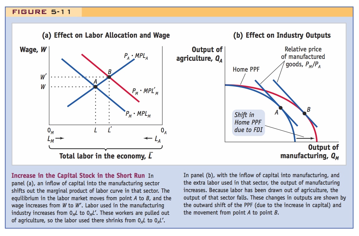
Effect of FDI on the Wage As a result of this shift, the equilibrium wage increases, from W to W′. More workers are drawn into the manufacturing industry, and the labor used there increases from 0ML to 0ML′. Because these workers are pulled out of agriculture, the labor used there shrinks from 0AL to 0AL′ (measuring from right to left).
146
Effect of FDI on the Industry Outputs It is easy to determine the effect of an inflow of FDI on industry outputs. Because workers are pulled out of agriculture, and there is no change in the amount of land used there, output of the agriculture industry must fall. With an increase in the number of workers used in manufacturing and an increase in capital used there, the output of the manufacturing industry must rise. These changes in output are shown in panel (b) of Figure 5-11 by the outward shift of the production possibilities frontier. At constant prices for goods (i.e., the relative price lines have the same slope before and after the increase in capital), the equilibrium outputs shift from point A to point B, with more manufacturing output and less agricultural output.
Effect of FDI on the Rentals Finally, we can determine the impact of the inflow of capital on the rental earned by capital and the rental earned by land. It is easiest to start with the agriculture industry. Because fewer workers are employed there, each acre of land cannot be cultivated as intensively as before, and the marginal product of land must fall. One way to measure the rental on land T is by the value of its marginal product, RT = PA · MPTA. With the fall in the marginal product of land (MPTA), and no change in the price of agricultural goods, the rental on land falls.
Now let us consider manufacturing, which uses more capital and more labor than before. One way to measure the rental on capital is by the value of the marginal product of capital, or RK = PM · MPKM. Using this method, however, it is difficult to determine how the rental on capital changes. As capital flows into manufacturing, the marginal product of capital falls because of diminishing returns. That effect reduces the rental on capital. But as labor is drawn into manufacturing, the marginal product of capital tends to rise. So we do not know at first glance how the rental on capital changes overall.
Fortunately, we can resolve this difficulty by using another method to measure the rental on capital. We take the revenue earned in manufacturing and subtract the payments to labor. If wages are higher, and everything else is the same, then there must be a reduced amount of funds left over as earnings of capital, so the rental is lower.
This is an elegant little argument, but be prepared to go through it step by step, slowly.
Let us apply this line of reasoning more carefully to see how the inflow of FDI affects the rental on capital. In Figure 5-12, we begin at point A and then assume the capital stock expands because of FDI. Suppose we hold the wage constant, and let the labor used in manufacturing expand up to point C. Because the wage is the same at points A and C, the marginal product of labor in manufacturing must also be the same (since the wage is W = PM · MPLM). The only way that the marginal product of labor can remain constant is for each worker to have the same amount of capital to work with as he or she had before the capital inflow. In other words, the capital–labor ratio in manufacturing LM/KM must be the same at points A and C: the expansion of capital in manufacturing is just matched by a proportional expansion of labor into manufacturing. But if the capital–labor ratio in manufacturing is identical at points A and C, then the marginal product of capital must also be equal at these two points (because each machine has the same number of people working on it). Therefore, the rental on capital, RK = PM · MPKM, is also equal at points A and C.
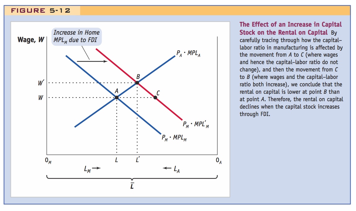
Now let’s see what happens as the manufacturing wage increases while holding constant the amount of capital used in that sector. The increase in the wage will move us up the curve  from point C to point B. As the wage rises, less labor is used in manufacturing. With less labor used on each machine in manufacturing, the marginal product of capital and the rental on capital must fall. This result confirms our earlier reasoning: when wages are higher and the amount of capital used in manufacturing is the same, then the earnings of capital (i.e., its rental) must be lower. Because the rental on capital is the same at points A and C but is lower at point B than C, the overall effect of the FDI inflow is to reduce the rental on capital. We learned previously that the FDI inflow also reduces the rental on land, so both rentals fall.
147
FDI in the Long Run
Say that we are really just applying Rybczynski again.
The results of FDI in the long run, when capital and labor can move between industries, differ from those we saw in the short-run specific-factors model. To model FDI in the long run, we assume again that there are two industries—computers and shoes—both of which use two factors of production: labor and capital. Computers are capital-intensive as compared with shoes, meaning that KC/LC exceeds KS/LS.
In panel (a) of Figure 5-13, we show the initial allocation of labor and capital between the two industries at point A. The labor and capital used in the shoe industry are 0SL and 0SK, so this combination is measured by the line 0SA. The labor and capital used in computers are 0CL and 0CK, so this combination is measured by the line 0CA. That amount of labor and capital used in each industry produces the output of shoes and computers shown by point A on the PPF in panel (b).
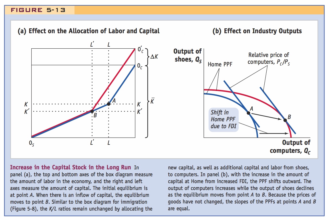
Effect of FDI on Outputs and Factor Prices An inflow of FDI causes the amount of capital in the economy to increase. That increase expands the right and left sides of the box in panel (a) of Figure 5-13 and shifts the origin up to  . The new allocation of factors between the industries is shown at point B. Now the labor and capital used in the shoe industry are measured by 0SB, which is shorter than the line 0SA. Therefore, less labor and less capital are used in the production of footwear, and shoe output falls. The labor and capital used in computers are measured by
  , which is longer than the line 0CA. Therefore, more labor and more capital are used in computers, and the output of that industry rises.
148
The change in outputs of shoes and computers is shown by the shift from point A to point B in panel (b) of Figure 5-13. In accordance with the Rybczynski theorem, the increase in capital through FDI has increased the output of the capital-intensive industry (computers) and reduced the output of the labor-intensive industry (shoes). Furthermore, this change in outputs is achieved with no change in the capital–labor ratios in either industry: the lines and 0SB have the same slopes as 0CA and 0SA, respectively.
Because the capital–labor ratios are unchanged in the two industries, the wage and the rental on capital are also unchanged. Each person has the same amount of capital to work with in his or her industry, and each machine has the same number of workers. The marginal products of labor and capital are unchanged in the two industries, as are the factor prices. This outcome is basically the same as that for immigration in the long run: in the long-run model, an inflow of either factor of production will leave factor prices unchanged.
When discussing immigration, we found cases in which wages were reduced (the short-run prediction) and other cases in which wages have been constant (the long-run prediction). What about for foreign direct investment? Does it tend to lower rentals or leave them unchanged? There are fewer studies of this question, but we next consider an important application for Singapore.
149
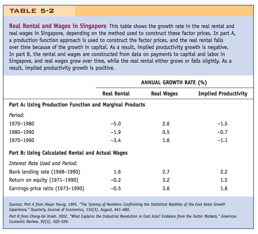
Singapore has aggressively attracted FDI. At first glance, it looks like rentals have decreased and wages have increased, as predicted by specific-factors. Using another method of calculating the rental, it has not fallen, but real wages have increased. This could be explained by productivity growth, but there is disagreement over whether it occurred.
The Effect of FDI on Rentals and Wages in Singapore
For many years, Singapore has encouraged foreign firms to establish subsidiaries within its borders, especially in the electronics industry. For example, many hard disks are manufactured in Singapore by foreign companies. In 2005 Singapore had the fourth largest amount of FDI in the world (measured by stock of foreign capital found there), following China, Mexico, and Brazil, even though it is much smaller than those economies.12 As capital in Singapore has grown, what has happened to the rental and to the wage?
One way to answer this question is to estimate the marginal product of capital in Singapore, using a production function that applies to the entire economy. The overall capital–labor ratio in Singapore has grown by about 5% per year from 1970 to 1990. Because of diminishing returns, it follows that the marginal product of capital (equal to the real rental) has fallen, by an average of 3.4% per year as shown in part A of Table 5-2. At the same time, each worker has more capital to work with, so the marginal product of labor (equal to the real wage) has grown by an average of 1.6% per year, as also shown in part A. These estimates of the falling rental and rising wage are consistent with the short-run specific-factors model.
150
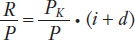
But there is a second way to calculate a rental on capital besides using the marginal product. Under this second approach, we start with the price PK of some capital equipment. If that equipment were rented rather than purchased, what would its rental be? Let us suppose that the rental agency needs to make the same rate of return on renting the capital equipment that it would make if it invested its money in some financial asset, such as a savings account in a bank or the stock market. If it invested PK and the asset had the interest rate of i, then it could expect to earn PK · i from that asset. On the other hand, if it rents out the equipment, then that machinery also suffers wear and tear, and the rental agency needs to recover that cost, too. If d is the rate of depreciation of the capital equipment (the fraction of it that is used up each year), then to earn the same return on a financial asset as from renting out the equipment, the rental agency must receive PK · (i + d). This formula is an estimate of R, the rental on capital. Dividing by an overall price index P, the real rental is
In part B of Table 5-2, we show the growth rate in the real rental, computed from this formula, which depends on the interest rate used. In the first row, we use the bank lending rate for i, and the computed real rental grows by 1.6% per year. In the next rows, we use two interest rates from the stock market: the return on equity (what you would earn from investing in stocks) and the earnings–price ratio (the profits that each firm earns divided by the value of its outstanding stocks). In both these latter cases, the calculated real rental falls slightly over time, by 0.2% and 0.5% per year, much less than the fall in the real rental in part A. According to the calculated real rentals in part B, there is little evidence of a downward fall in the rentals over time.
In part B, we also show the real wage, computed from actual wages paid in Singapore. Real wages grow substantially over time—between 2.7% and 3.6% per year, depending on the exact interest rate and period used. This is not what we predicted from our long-run model, in which factor prices would be unchanged by an inflow of capital, because the capital–labor ratios are constant (so the marginal product of labor would not change). That real wages are growing in Singapore, with little change in the real rental, is an indication that there is productivity growth in the economy, which leads to an increase in the marginal product of labor and in the real wage.
We will not discuss how productivity growth is actually measured13 but just report the findings from the studies in Table 5-2: in part B, productivity growth is between 1.5% and 2.2% per year, depending on the period, but in part A, productivity growth is negative! The reason that productivity growth is so much higher in part B is because the average of the growth in the real wage and real rental is rising, which indicates that productivity growth has occurred. In contrast, in part A the average of the growth in the real wage and real rental is zero or negative, indicating that no productivity growth has occurred.
The idea that Singapore might have zero productivity growth contradicts what many people believe about its economy and the economies of other fast-growing Asian countries, which were thought to exhibit “miraculous” growth during this period. If productivity growth is zero or negative, then all growth is due only to capital accumulation, and FDI has no spillover benefits to the local economy. Positive productivity growth, as shown in part B, indicates that the free-market policies pursued by Singapore stimulated innovations in the manufacture of goods that have resulted in higher productivity and lower costs. This is what many economists and policy makers believe happened in Singapore, but this belief is challenged by the productivity calculations in part A. Which scenario is correct—zero or positive productivity growth for Singapore—is a source of ongoing debate in economics. Read the item Headlines: The Myth of Asia’s Miracle for one interpretation of the growth in Singapore and elsewhere in Asia.
151