1 Basics of Imperfect Competition
1. Objective: Review monopoly and demand under duopoly
2. Monopoly Equilibrium
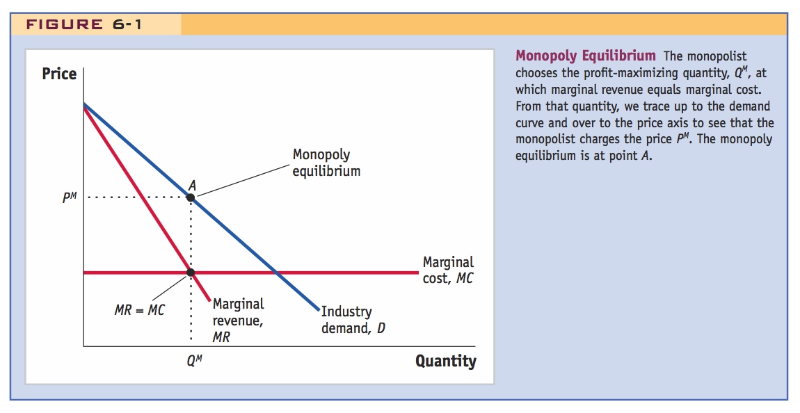
Given industry demand D, derive MR. Assume constant MC. Maximize profit when MR = MC, so P > MC.
3. Demand with Duopoly
Won’t solve for duopoly equilibrium, just look at how the existence of a second firm affects the demand faced by both: If both firms set the same price, then the demand curve faced by each is just half of the industry demand (D/2). If one firm sets a lower price, however, it raises its quantity demanded by more, since it steals demand from the other firm. Therefore, the demand curve of each firm in a duopoly is more elastic than D/2, when both firms set the same price.
Monopolistic competition incorporates some aspects of a monopoly (firms have control over the prices they charge) and some aspects of perfect competition (many firms are selling). Before presenting the monopolistic competition model, it is useful to review the case of monopoly, which is a single firm selling a product. The monopoly firm faces the industry demand curve. After that, we briefly discuss the case of duopoly, when there are two firms selling a product. Our focus will be on the demand facing each of the two firms. Understanding what happens to demand in a duopoly will help us understand how demand is determined when there are many firms selling differentiated products, as occurs in monopolistic competition.
Monopoly Equilibrium
They will probably be familiar with this, so a quick review will suffice. Maybe add something about the markup and elasticity.
In Figure 6-1, the industry demand curve is shown by D. For the monopolist to sell more, the price must fall, and so the demand curve slopes downward. This fall in price means that the extra revenue earned by the monopolist from selling another unit is less than the price of that unit—the extra revenue earned equals the price charged for that unit minus the fall in price times the quantity sold of all earlier units. The extra revenue earned from selling one more unit is called the marginal revenue and is shown by the curve MR in Figure 6-1. The marginal revenue curve lies below the demand curve D because the extra revenue earned from selling another unit is less than the price.
169
To maximize its profit, the monopolist sells up to the point at which the marginal revenue MR earned from selling one more unit equals the marginal cost MC of producing one more unit. In Figure 6-1, the marginal cost curve is shown by MC. Because we have assumed, for simplicity, that marginal costs are constant, the MC curve is flat, although this does not need to be the case. To have marginal revenue equal marginal costs, the monopolist sells the quantity QM. To find the profit-maximizing price the monopolist charges, we trace up from quantity QM to point A on the demand curve and then over to the price axis. The price charged by the monopolist PM is the price that allows the monopolist to earn the highest profit and is therefore the monopoly equilibrium.
Demand with Duopoly
It is not too clear at first whether this price or quantity competition, but implicitly it is Bertrand competition with differentiated products. Call it that, since some students will have encountered it.
Let us compare a monopoly with a duopoly, a market structure in which two firms are selling a product. We will not solve for the duopoly equilibrium but will just study how the introduction of a second firm affects the demand facing each of the firms. Knowing how demand is affected by the introduction of a second firm helps us understand how demand is determined when there are many firms, as there are in monopolistic competition.
In Figure 6-2, the industry faces the demand curve D. If there are two firms in the industry and they charge the same price, then the demand curve facing each firm is D/2. For example, if both firms charged the price P1, then the industry demand is at point A, and each firm’s demand is at point B on curve D/2. The two firms share the market equally, each selling exactly one-half of the total market demand, Q2 = Q1/2.
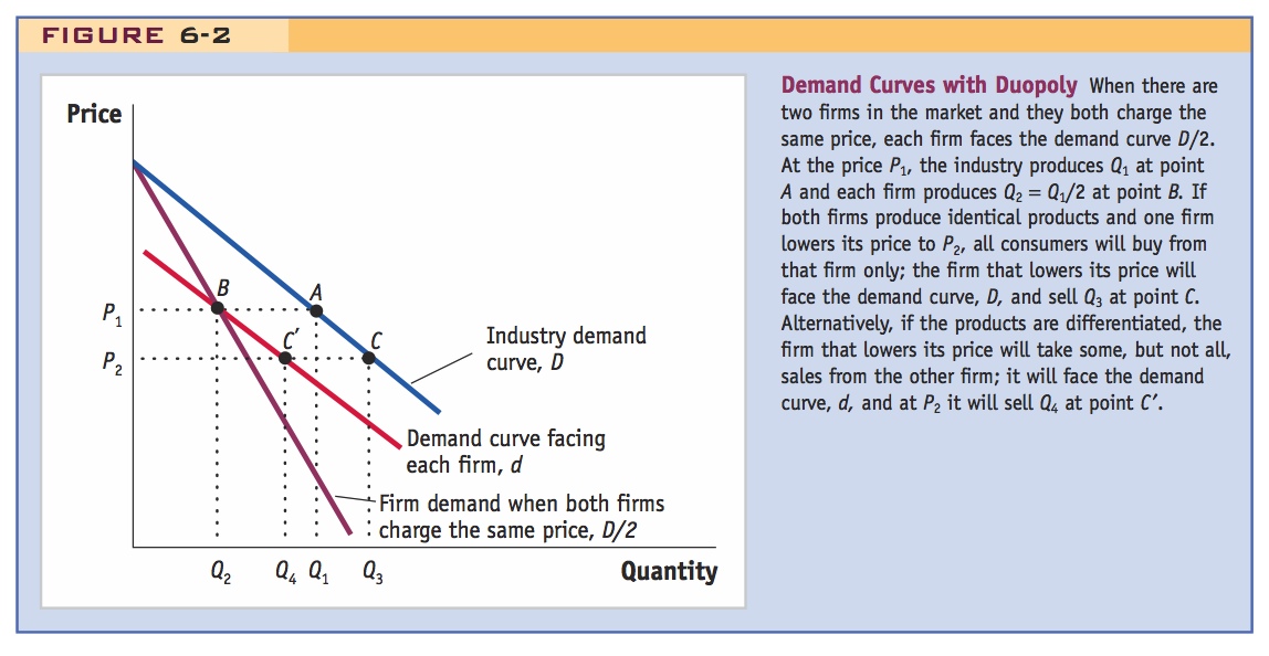
If one firm charges a price different from the other firm, however, the demand facing both firms changes. Suppose that one firm charges a lower price P2, while the other firm keeps its price at P1. If the firms are selling the same homogeneous product, then the firm charging the lower price would get all the demand (shown by point C), which is Q3 at the price P2. Now suppose that the products are not homogeneous but instead are differentiated. In that case, the firm with the lower price P2 will capture more of the market than the firm with the higher price P1, but will not capture the entire market. Because the products are not precisely the same (for instance, in our golf club example the higher-priced club is of better quality than the less expensive club), some consumers will still want to buy the other firm’s product even though its price is higher. The firm selling at the lower price P2 now sells the quantity Q4, for example, at point C′.
170
Make sure students grasp this, since it is crucial in what follows.
The demand curve d is the demand curve for the firm that lowered its price from P1 to P2, even though the other firm held its price at P1. As we have illustrated, the demand curve d is flatter than the demand curve D/2. This means that each firm faces a more elastic demand curve than D/2: when only one firm lowers its price, it increases its quantity sold by more than when all firms lower their prices. Not only does the quantity demanded in the industry increase, but in addition, the firm that lowers its price takes away some of the quantity demanded from the other firm. In summary, the demand curve d facing each firm producing in a duopoly is more elastic than the demand curve D/2 each faces when the firms charge the same price.