2 Trade Under Monopolistic Competition

We begin our study of monopolistic competition by carefully stating the assumptions of the model.

Assumption 1: Each firm produces a good that is similar to but differentiated from the goods that other firms in the industry produce.

Because each firm’s product is somewhat different from the goods of the other firms, a firm can raise its price without losing all its customers to other firms. Thus, each firm faces a downward-sloping demand curve for its product and has some control over the price it charges. This is different from perfect competition, in which all firms produce exactly the same product and therefore must sell at exactly the same market-determined price.

Assumption 2: There are many firms in the industry.

The discussion of duopoly demand in the previous section helps us to think about the demand curve facing a firm under monopolistic competition, when there are many firms in the industry. If the number of firms is N, then D/N is the share of demand that each firm faces when the firms are all charging the same price. When only one firm lowers its price, however, it will face a flatter demand curve d. We will begin describing the model by focusing on the demand curve d and later bring back the demand curve D/N.

The first two assumptions are about the demand facing each firm; the third assumption is about each firm’s cost structure:

Assumption 3: Firms produce using a technology with increasing returns to scale.

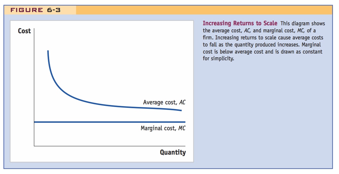
The assumptions underlying monopolistic competition differ from our usual assumptions on firm costs by allowing for increasing returns to scale, a production technology in which the average costs of production fall as the quantity produced increases. This relationship is shown in Figure 6-3, in which average costs are labeled AC. The assumption that average costs fall as quantity increases means that marginal costs, labeled MC, must be below average costs. Why? Think about whether a new student coming into your class will raise or lower the class average grade. If the new student’s average is below the existing class average, then when he or she enters, the class average will fall. In the same way, when MC is less than AC, then AC must be falling.3

Numerical Example As an example of the cost curves in Figure 6-3, suppose that the firm has the following cost data:

Given these costs, the average costs for this firm for various quantities are as shown in Table 6-2.

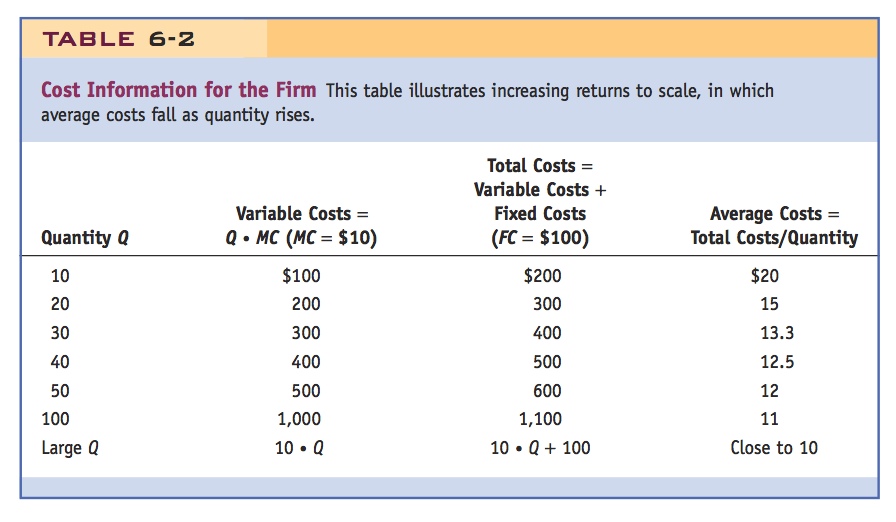
Notice that as the quantity produced rises, average costs fall and eventually become close to the marginal costs of $10 per unit, as shown in Figure 6-3.

Assumption 3 means that average cost is above marginal cost. Assumption 1 means that firms have some control over the price they charge, and these firms charge a price that is also above marginal cost (we learn why in a later section).

Whenever the price charged is above average cost, a firm earns monopoly profit. Our final assumption describes what happens to profits in a monopolistically competitive industry in the long run:

Assumption 4: Because firms can enter and exit the industry freely, monopoly profits are zero in the long run.

Recall that under perfect competition, we assume there are many firms in the industry and that in a long-run equilibrium each firm’s profit must be zero. In monopolistic competition, there is the same requirement for a long-run equilibrium. We assume that firms can enter and exit the industry freely; this means that firms will enter as long as it is possible to make monopoly profits, and as more firms enter, the profit per firm falls. This condition leads to a long-run equilibrium in which profit for each firm is zero, just as in perfect competition!

Equilibrium Without Trade

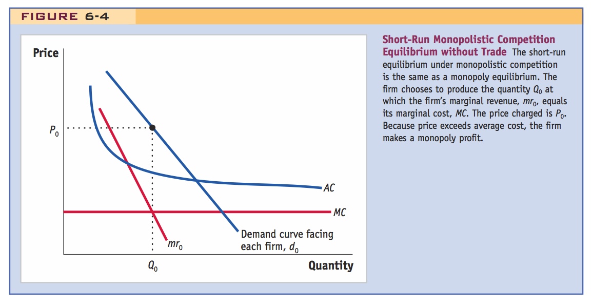
Short-Run Equilibrium The short-run equilibrium for a firm under monopolistic competition, shown in Figure 6-4, is similar to a monopoly equilibrium. The demand curve faced by each firm is labeled d₀, the marginal revenue curve is labeled mr₀, and the marginal cost curve of each firm is shown by MC. Each firm maximizes profit by producing Q₀, the quantity at which marginal revenue equals marginal cost. Tracing up from this quantity to the demand curve shows that the price charged by the firms is P₀. Because the price exceeds average costs at the quantity Q₀, the firm earns monopoly profit.

Long-Run Equilibrium In a monopolistically competitive market, new firms continue to enter the industry as long as they can earn monopoly profits. In the long run, the entry of new firms draws demand away from existing firms, causing demand curve d₀ to shift to the left until no firm in the industry earns positive monopoly profits (Figure 6-5). Moreover, when new firms enter and there are more product varieties available to consumers, the d₀ curve faced by each firm becomes more elastic, or flatter. We expect the d₀ curve to become more elastic as more firms enter because each product is similar to the other existing products; therefore, as the number of close substitutes increases, consumers become more price sensitive.

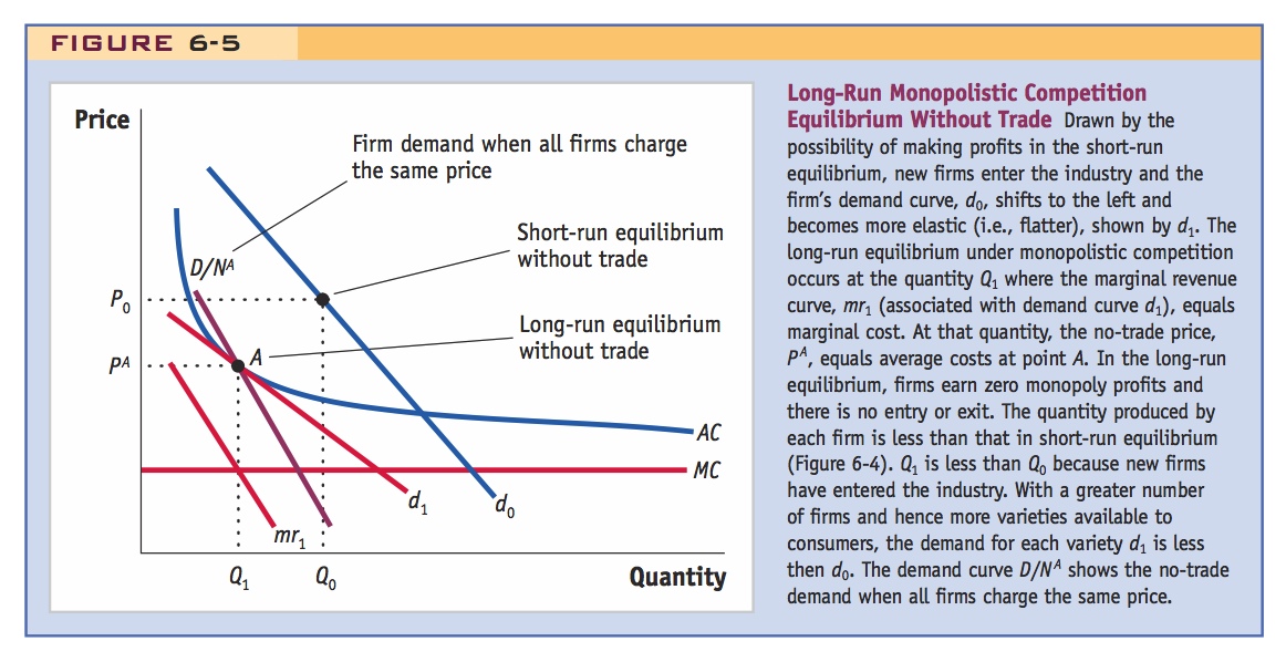
New firms continue to enter the industry until the price charged by each firm is on the average cost curve and monopoly profit is zero. At this point, the industry is in a long-run equilibrium, with no reason for any further entry or exit. The long-run equilibrium without trade is shown in Figure 6-5. Again, the demand curve for the firm is labeled d, with the short-run demand curve denoted d₀ and the long-run demand curve denoted d₁ (with corresponding marginal revenue curve mr₁). Marginal revenue equals marginal cost at quantity Q₁. At this quantity, all firms in the industry charge price P^A. The price P ^A equals average cost at point A, where the demand curve d₁ is tangent to the average cost curve. Because the price equals average costs, the firm is earning zero monopoly profit and there is no incentive for firms to enter or exit the industry. Thus, point A is the firm’s (and the industry’s) long-run equilibrium without trade. Notice that the long-run equilibrium curve d₁ is to the left of and more elastic (flatter) than the short-run curve d₀.

Before we allow for international trade, we need to introduce another curve into Figure 6-5. The firm’s demand curve d₁ shows the quantity demanded depending on the price charged by that firm, holding the price charged by all other firms fixed. In contrast, there is another demand curve that shows the quantity demanded from each firm when all firms in the industry charge the same price. This other demand curve is the total market demand D divided by the number of firms in the absence of trade N ^A. In Figure 6-5, we label the second demand curve as D/N^A. We omit drawing total industry demand D itself so we do not clutter the diagram.

The demand curve d₁ is flatter, or more elastic, than the demand curve D/N^A. We discussed why that is the case under duopoly (see Figure 6-2) and can review the reason again now. Starting at point A, consider a drop in the price by just one firm, which increases the quantity demanded along the d₁ curve for that firm. The demand curve d₁ is quite elastic, meaning that the drop in price leads to a large increase in the quantity purchased because customers are attracted away from other firms. If instead all firms drop their price by the same amount, along the curve D/N^A, then each firm will not attract as many customers away from other firms. When all firms drop their prices equally, then the increase in quantity demanded from each firm along the curve D/N^A is less than the increase along the firm’s curve d₁. Thus, demand is less elastic along the demand curve D/N^A, which is why it is steeper than the d₁ curve. As we proceed with our analysis of opening trade under monopolistic competition, it will be helpful to keep track of both of these demand curves.

Equilibrium with Free Trade

Let us now allow for free trade between Home and Foreign in this industry. For simplicity, we assume that Home and Foreign countries are exactly the same, with the same number of consumers, the same factor endowments, the same technology and cost curves, and the same number of firms in the no-trade equilibrium. If there were no increasing returns to scale, there would be no reason at all for international trade to occur. Under the Ricardian model, for example, countries with identical technologies would not trade because their no-trade relative prices would be equal. Likewise, under the Heckscher-Ohlin model, countries with identical factor endowments would not trade because their no-trade relative prices would be the same. Under monopolistic competition, however, two identical countries will still engage in international trade because increasing returns to scale exist.

Short-Run Equilibrium with Trade We take as given the number of firms in the no-trade equilibrium in each country N^A and use this number of firms to determine the short-run equilibrium with trade. Our starting point is the long-run equilibrium without trade, as shown by point A in Figure 6-5 and reproduced in Figure 6-6. When we allow free trade between Home and Foreign, the number of consumers available to each firm doubles (because there is an equal number of consumers in each country) as does the number of firms (because there is an equal number of firms in each country). Because there are not only twice as many consumers but also twice as many firms, the demand curve D/N^A is the same as it was before, 2D/2N^A = D/N^A. In other words, point A is still on the demand curve D/N^A, as shown in Figure 6-6.

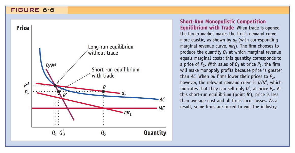
Free trade doubles the number of firms, which also doubles the product varieties available to consumers. With a greater number of product varieties available to consumers, their demand for each individual variety will be more elastic. That is, if one firm drops its price below the no-trade price P ^A, then it can expect to attract an even greater number of customers away from other firms. Before trade the firm would attract additional Home customers only, but after trade it will attract additional Home and Foreign consumers. In Figure 6-6, this consumer response is shown by the firm’s new demand curve d₂, which is more elastic than its no-trade demand curve d₁. As a result, the demand curve d₂ is no longer tangent to the average cost curve at point A but is above average costs for prices below P ^A. The new demand curve d₂ has a corresponding marginal revenue curve mr₂, as shown in Figure 6-6.

With the new demand curve d₂ and new marginal revenue curve mr₂, the firm again needs to choose its profit-maximizing level of production. As usual, that level will be where marginal revenue equals marginal cost at Q₂. When we trace from Q₂ up to point B on the firm’s demand curve d₂, then over to the price axis, we see that the firm will charge P₂. Because P₂ is above average cost at point B, the firm will make a positive monopoly profit. We can see clearly the firm’s incentive to lower its price: at point A it earns zero monopoly profit and at point B it earns positive profit. Producing Q₂ and selling it at P₂ is the firm’s profit-maximizing position.

This happy scenario for the firm is not the end of the story, however. Every firm in the industry (in both Home and Foreign) has the same incentive to lower its price in the hope of attracting customers away from all the other firms and earning monopoly profit. When all firms lower their prices at the same time, however, the quantity demanded from each firm increases along the demand curve D/N ^A, not along d₂. Remember that the D/N ^A curve shows the demand faced by each firm when all firms in the industry charge the same price. With the prices of all firms lowered to P₂, they will each sell the quantity Q′₂ at point B′ rather than their expected sales of Q₂ at point B. At point B′, the price charged is less than average costs, so every firm is incurring a loss. In the short-run equilibrium with trade, firms lower their prices, expecting to make profits at point B, but end up making losses at point B′.

Point B′ is not the long-run equilibrium because the losses will bankrupt some firms and cause them to exit from the industry. This exit will increase demand (both d and D/N ^A) for the remaining firms and decrease the number of product varieties available to consumers. To understand where the new long-run equilibrium occurs, we turn to a new diagram.

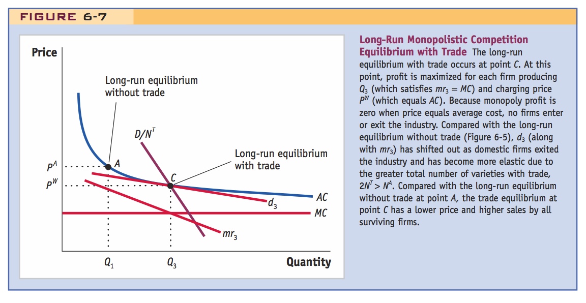
Long-Run Equilibrium with Trade Due to the exit of firms, the number of firms remaining in each country after trade is less than it was before trade. Let us call the number of firms in each country after trade is opened N^T, where N^T < N^A. This reduction in the number of firms increases the share of demand facing each one, so that D/N^T > D/N^A. In Figure 6-7, the demand D/N^T facing each firm lies to the right of the demand D/N^A in the earlier figures. We show the long-run equilibrium with trade at point C. At point C, the demand curve d₃ facing an individual firm is tangent to the average cost curve AC. In addition, the marginal revenue curve mr₃ intersects the marginal cost curve MC.

How does this long-run equilibrium compare to that without trade? First of all, despite the exit of some firms in each country, we still expect that the world number of products, which is 2N^T (the number produced in each country N^T times two countries), exceeds the number of products N^A available in each country before trade, 2N^T > N^A. It follows that the demand curve d₃ facing each firm must be more elastic than demand d₁ in the absence of trade: the availability of imported products makes consumers more price sensitive than they were before trade, so the demand curve d₃ is more elastic than demand d₁ in Figure 6-5. At free-trade equilibrium (point C), each firm still in operation charges a lower price than it did with no trade, P^W < P^A, and produces a higher quantity, Q₃ > Q₁. The drop in prices and increase in quantity for each firm go hand in hand: as the quantity produced by each surviving firm increases, average costs fall due to increasing returns to scale, and so do the prices charged by firms.

Gains from Trade The long-run equilibrium at point C has two sources of gains from trade for consumers. First, the price has fallen as compared with point A, so consumers benefit for that reason. A good way to think about this drop in the price is that it reflects increasing returns to scale, with average costs falling as the output of firms rises. The drop in average costs is a rise in productivity for these surviving firms because output can be produced more cheaply. So consumers gain from the drop in price, which is the result of the rise in productivity.

There is a second source of gains from trade to consumers. We assume that consumers obtain higher surplus when there are more product varieties available to buy, and hence the increase in variety is a source of gain for consumers. Within each country, some firms exit the market after trade begins, so fewer product varieties are produced by the remaining domestic firms. However, because consumers can buy products from both Home and Foreign firms, the total number of varieties available with trade is greater than the number of varieties available in any one country before trade, 2N^T > N^A. Thus, in addition to the drop in prices, there is an added consumer gain from the availability of additional product varieties.

Adjustment Costs from Trade Against these long-run gains from trade, there are short-run adjustment costs as some firms in each country shut down and exit the industry. The workers in those firms will experience a spell of unemployment as they look for new jobs. Over the long run, however, we expect these workers to find new positions, so we view these costs as temporary. We do not build these adjustment costs into the model because they are short-term, but we are still interested in how large these costs might be in practice. To compare the short-run adjustment costs with the long-run gains from trade, we next look at the evidence from Canada, Mexico, and the United States under the North American Free Trade Agreement. We will see that the predictions of the monopolistic competition model hold reasonably well in each case.