3 Import Tariffs for a Small Country
Distinguish between specific and ad valorem tariffs.
The tariff is a tax levied at the border, so consumer prices increase by the amount of the tariff.
1. Free Trade for a Small Country
Foreign export supply is perfectly elastic at the world price, which determines the imports.
2. Effect of the Tariff
Foreign export supply shifts up by the amount of the tariff, so imports fall: The increase in the import price also raises the price of the good produced domestically, since the good is homogeneous. Quantity demanded falls and quantity supplied increases, so imports decrease.
a. Effect of the Tariff on Consumer Surplus
Consumers pay more per unit for a smaller quantity, so consumer surplus falls.
b. Effect of the Tariff on Producer Surplus
Revenues increase more than costs, so producer surplus increases.
c. Effect of the Tariff on Government Revenue
The government gets revenue equal to tariff x imports, a gain to the economy.
d. Overall Effect of the Tariff on Welfare
Calculate the deadweight loss. Interpretation:
e. Production Loss
Results from the fact that every unit of the increased production is at a price in excess of MC, so the economy is producing inefficiently.
f. Consumption Loss
Results from the fact that some consumers have to reduce consumption of the good because of the higher price.
3. Why and How Are Tariffs Applied?
If tariffs have deadweight losses, why do countries use them? Two answers: First, other types of taxes might be hard to collect, especially in developing countries. Tariffs have the virtue of being easy to collect. Second, the costs of tariffs are spread around many consumers, while the benefits might be concentrated on a small number of producers. So producers may exert political pressure to lobby for tariffs. Examples: Obama’s tire tariff and Bush’s steel tariff.
We can now use this supply and demand framework to show what happens when a small country imposes a tariff. As we have already explained, an importing country is “small” if its tariff does not have any effect on the world price of the good on which the tariff is applied. As we will see, the Home price of the good will increase due to the tariff. Because the tariff (which is a tax) is applied at the border, the price charged to Home consumers will increase by the amount of the tariff.
Free Trade for a Small Country
In Figure 8-4, we again show the free-trade equilibrium for the Home country. In panel (b), the Foreign export supply curve X* is horizontal at the world price PW. The horizontal export supply curve means that Home can import any amount at the price PW without having an impact on that price. The free-trade equilibrium is determined by the intersection of the Foreign export supply and the Home import demand curves, which is point B in panel (b), at the world price PW. At that price, Home demand is D1 and Home supply is S1, shown in panel (a). Imports at the world price PW are then just the difference between demand and supply, or M1 = D1 − S1.
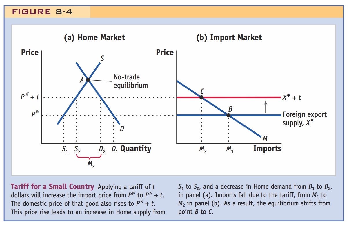
Effect of the Tariff
With the import tariff of t dollars, the export supply curve facing the Home country shifts up by exactly that amount, reflecting the higher price that must be paid to import the good. The shift in the Foreign export supply curve is analogous to the shift in domestic supply caused by a sales tax, as you may have seen in earlier economics courses; it reflects an effective increase in the costs of the firm. In panel (b) of Figure 8-4, the export supply curve shifts up to X* + t. The intersection of the post-tariff export supply curve and the import demand curve now occurs at the price of PW + t and the import quantity of M2. The import tariff has reduced the amount imported, from M1 under free trade to M2 under the tariff, because of its higher price.
243
Remind students of the assumptions of perfect competition.
We assume that the imported product is identical to the domestic alternative that is available. For example, if the imported product is a women’s cruiser bicycle, then the Home demand curve D in panel (a) is the demand for women’s cruisers, and the Home supply curve is the supply of women’s cruisers. When the import price rises to PW + t, then we expect that the Home price for locally produced bicycles will rise by the same amount. This is because at the higher import price of PW + t, the quantity of cruisers demanded at Home falls from its free-trade quantity of D1 to D2. At the same time, the higher price will encourage Home firms to increase the quantity of cruisers they supply from the free-trade quantity of S1 to S2. As firms increase the quantity they produce, however, the marginal costs of production rise. The Home supply curve (S) reflects these marginal costs, so the Home price will rise along the supply curve until Home firms are supplying the quantity S2, at a marginal cost just equal to the import price of PW + t. Since marginal costs equal PW + t, the price charged by Home firms will also equal PW + t, and the domestic price will equal the import price.
Summing up, Home demand at the new price is D2, Home supply is S2, and the difference between these are Home imports of M2 = D2 − S2. Foreign exporters still receive the “net-of-tariff” price (i.e., the Home price minus the tariff) of PW, but Home consumers pay the higher price PW + t. We now investigate how the rise in the Home price from PW to PW + t affects consumer surplus, producer surplus, and overall Home welfare.
244
This is traditionally called the "consumption effect."
Effect of the Tariff on Consumer Surplus In Figure 8-5, we again show the effect of the tariff of t dollars, which is to increase the price of the imported and domestic good from PW to PW + t. Under free trade, consumer surplus in panel (a) was the area under the demand curve and above PW. With the tariff, consumers now pay the higher price, PW + t, and their surplus is the area under the demand curve and above the price PW + t. The fall in consumer surplus due to the tariff is the area between the two prices and to the left of Home demand, which is (a + b + c + d) in panel (a) of Figure 8-5. This area is the amount that consumers lose due to the higher price caused by the tariff.

Likewise, "production effect."
Effect of the Tariff on Producer Surplus We can also trace the impact of the tariff on producer surplus. Under free trade, producer surplus was the area above the supply curve in panel (a) and below the price of PW. With the tariff, producer surplus is the area above the supply curve and below the price PW + t: since the tariff increases the Home price, firms are able to sell more goods at a higher price, thus increasing their surplus. We can illustrate this rise in producer surplus as the amount between the two prices and to the left of Home supply, which is labeled as a in panel (a). This area is the amount that Home firms gain because of the higher price caused by the tariff. As we have just explained, the rise in producer surplus should be thought of as an increase in the return to fixed factors (capital or land) in the industry. Sometimes we even think of labor as a partially fixed factor because the skills learned in one industry cannot necessarily be transferred to other industries. In that case, it is reasonable to think that the increase in Home producer surplus can also benefit Home workers in the import-competing industry, along with capital and land, but this benefit comes at the expense of consumer surplus.
And "revenue effect."
Some students will ask why government revenue is a gain. Argue that it may be spent on goods of this value, or argue that in principle it could redistribute it back to consumers, partially compensating them for their loses. The main point is that the pie is smaller, with or without the government revenues.
Effect of the Tariff on Government Revenue In addition to affecting consumers and producers, the tariff also affects government revenue. The amount of revenue collected is the tariff t times the quantity of imports (D2 − S2). In Figure 8-5, panel (a), this revenue is shown by the area c. The collection of revenue is a gain for the government in the importing country.
We don't care, because this is a measure of the increase in the size of the pie, and are agnostic about how it is shared.
Overall Effect of the Tariff on Welfare We are now in a position to summarize the impact of the tariff on the welfare of the Home importing country, which is the sum of producer surplus, consumer surplus, and government revenues. Thus, our approach is to add up these impacts to obtain a net effect. In adding up the loss of consumers and the gains of producers, one dollar of consumer surplus is the same as one dollar of producer surplus or government revenue. In other words, we do not care whether the consumers facing higher prices are poor or rich, and do not care whether the specific factors in the industry (capital, land, and possibly labor) earn a lot or a little. Under this approach, transferring one dollar from consumer to producer surplus will have no impact on overall welfare: the decrease in consumer surplus will cancel out the increase in producer surplus.
Developing Pareto earlier allows this to be defined precisely.
You may object to this method of evaluating overall welfare, and feel that a dollar taken away from a poor consumer and given to a rich producer represents a net loss of overall welfare, rather than zero effect, as in our approach. We should be careful in evaluating the impact of tariffs on different income groups in the society, especially for poor countries or countries with a high degree of inequality among income groups. But for now we ignore this concern and simply add up consumer surplus, producer surplus, and government revenue. Keep in mind that under this approach we are just evaluating the efficiency of tariffs and not their effect on equity (i.e., how fair the tariff is to one group versus another).
245
Use the numerical example of free trade from before, add a tariff, and have them calculate all of these changes.
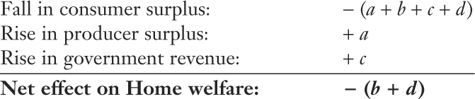
The overall impact of the tariff in the small country can be summarized as follows:
Ask the students to think about how the size of the deadweight loss changes with the price elasticities of domestic demand and supply.
In Figure 8-5(b), the triangle (b + d) is the net welfare loss in a small importing country due to the tariff. We sometimes refer to this area as a deadweight loss, meaning that it is not offset by a gain elsewhere in the economy. Notice that in panel (a) the area a, which is a gain for producers, just cancels out that portion of the consumer surplus loss; the area a is effectively a transfer from consumers to producers via the higher domestic prices induced by the tariff. Likewise, area c, the gain in government revenue, also cancels out that portion of the consumer surplus loss; this is a transfer from consumers to the government. Thus, the area (b + d) is the remaining loss for consumers that is not offset by a gain elsewhere. This deadweight loss is measured by the two triangles, b and d, in panel (a), or by the combined triangle (b + d) in panel (b). The two triangles b and d of deadweight loss can each be given a precise interpretation, as follows.
It is important to elaborate on the economic meaning of these triangles, since some students are prone to memorizing the pictures without understanding what they mean
Production Loss Notice that the base of triangle b is the net increase in Home supply due to the tariff, from S1 to S2. The height of this triangle is the increase in marginal costs due to the increase in supply. The unit S1 was produced at a marginal cost equal to PW, which is the free-trade price, but every unit above that amount is produced with higher marginal costs. The fact that marginal costs exceed the world price means that this country is producing the good inefficiently: it would be cheaper to import it rather than produce the extra quantity at home. The area of triangle b equals the increase in marginal costs for the extra units produced and can be interpreted as the production loss (or the efficiency loss) for the economy due to producing at marginal costs above the world price. Notice that the production loss is only a portion of the overall deadweight loss, which is (b + d) in Figure 8-5.
246
Consumption Loss The triangle d in panel (a) (the other part of the deadweight loss) can also be given a precise interpretation. Because of the tariff and the price increase from PW to PW + t, the quantity consumed at Home is reduced from D1 to D2. The area of the triangle d can be interpreted as the drop in consumer surplus for those individuals who are no longer able to consume the units between D1 and D2 because of the higher price. We refer to this drop in consumer surplus as the consumption loss for the economy.
Why and How Are Tariffs Applied?
Our finding that a tariff always leads to deadweight losses for a small importing country explains why most economists oppose the use of tariffs. If a small country suffers a loss when it imposes a tariff, why do so many have tariffs as part of their trade policies? One answer is that a developing country does not have any other source of government revenue. Import tariffs are “easy to collect” because every country has customs agents at major ports checking the goods that cross the border. It is easy to tax imports, even though the deadweight loss from using a tariff is typically higher than the deadweight loss from using “hard-to-collect” taxes, such as income taxes or value-added taxes. These taxes are hard to collect because they require individuals and firms to honestly report earnings, and the government cannot check every report (as they can check imports at the border). Still, to the extent that developing countries recognize that tariffs have a higher deadweight loss, we would expect that over time they would shift away from such easy-to-collect taxes. That is exactly what has occurred, according to one research study.4 The fraction of total tax revenue collected from “easy to collect” taxes such as tariffs fell during the 1980s and 1990s, especially in developing countries, whereas the fraction of revenue raised from “hard to collect” taxes rose over this same period.
A second reason why tariffs are used even though they have a deadweight loss is politics. The tariff benefits the Home producers, as we have seen, so if the government cares more about producer surplus than consumer surplus, it might decide to use the tariff despite the deadweight loss it incurs. Indeed, the benefits to producers (and their workers) are typically more concentrated on specific firms and states than the costs to consumers, which are spread nationwide. This is our interpretation of the tariff that President George W. Bush granted to the steel industry from 2002 to 2004: its benefits were concentrated in the steel-producing states of Pennsylvania, West Virginia, and Ohio, and its costs to consumers—in this case, steel-using industries—were spread more widely.5 For the tariff on tires imported from China granted by President Barack Obama from 2009 to 2012, the argument is a bit different. This tariff was requested by the United Steelworkers, the union who represents workers in the U.S. tire industry, and it was expected to benefit those workers. But U.S. tire producers did not support the tariff because many of them were already manufacturing tires in other countries—especially China—and this tariff made it more costly for them to do so.
247
In both the steel and tire cases, the president was not free to impose just any tariff, but had to follow the rules of the GATT discussed earlier in this chapter. Recall that Article XIX of the GATT, known as the “safeguard” or “escape clause,” allows a temporary tariff to be used under certain circumstances. GATT Article XIX is mirrored in U.S. trade law. In Side Bar: Safeguard Tariffs, we list the key passages for two sections of the Trade Act of 1974, as amended, both of which deal with safeguard tariffs.
First, Section 201 states that a tariff can be requested by the president, by the House of Representatives, by the Senate, or by any other party such as a firm or union that files a petition with the U.S. International Trade Commission (ITC). That commission determines whether rising imports have been “a substantial cause of serious injury, or threat thereof, to the U.S. industry….” The commission then makes a recommendation to the president who has the final authority to approve or veto the tariff. Section 201 goes further in defining a “substantial cause” as a “cause that is important and not less than any other cause.” Although this kind of legal language sounds obscure, it basically means that rising imports have to be the most important cause of injury to justify import protection. The steel tariff used by President Bush met this criterion, but as we see in later chapters, many other requests for tariffs do not meet this criterion and are not approved.
Both Obama and Bush had to justify their tariffs as “safeguard tariffs” to satisfy GATT and U.S. Trade law.
Safeguard Tariffs
The U.S. Trade Act of 1974, as amended, describes conditions under which tariffs can be applied in the United States, and it mirrors the provisions of the GATT and WTO. Two sections of the Trade Act of 1974 deal with the use of “safeguard” tariffs:
Section 201
Upon the filing of a petition…, the request of the President or the Trade Representative, the resolution of either the Committee on Ways and Means of the House of Representatives or the Committee on Finance of the Senate, or on its own motion, the [International Trade] Commission shall promptly make an investigation to determine whether an article is being imported into the United States in such increased quantities as to be a substantial cause of serious injury, or the threat thereof, to the domestic industry producing an article like or directly competitive with the imported article.
…For purposes of this section, the term “substantial cause” means a cause which is important and not less than any other cause.
Section 421
Upon the filing of a petition…the United States International Trade Commission…shall promptly make an investigation to determine whether products of the People’s Republic of China are being imported into the United States in such increased quantities or under such conditions as to cause or threaten to cause market disruption to the domestic producers of like or directly competitive products.
…(1) For purposes of this section, market disruption exists whenever imports of an article like or directly competitive with an article produced by a domestic industry are increasing rapidly, either absolutely or relatively, so as to be a significant cause of material injury, or threat of material injury, to the domestic industry.
(2) For purposes of paragraph (1), the term “significant cause” refers to a cause which contributes significantly to the material injury of the domestic industry, but need not be equal to or greater than any other cause.
Source: http://www.law.cornell.edu/uscode/text/19/2252 and www.law.cornell.edu/uscode/text/19/2451
248
A second, more recent amendment to the Trade Act of 1974 is Section 421 that applies only to China. This provision was added by the United States as a condition to China’s joining the WTO in 2001.6 Because the United States was worried about exceptional surges in imports from China, it drafted this legislation so that tariffs could be applied in such a case. Under Section 421, various groups can file a petition with the U.S. International Trade Commission, which makes a recommendation to the president. The commission must determine whether rising imports from China cause “market disruption” in a U.S. industry, which means “a significant cause of material injury, or threat of material injury, to the domestic industry.” Furthermore, the term “significant cause” refers to “a cause which contributes significantly to the material injury of the domestic industry, but need not be equal to or greater than any other cause.” Again, the legal language can be hard to follow, but it indicates that tariffs can be applied even when rising imports from China are not the most important cause of injury to the domestic industry. Section 421 can therefore be applied under weaker conditions than Section 201, and it was used by President Obama to justify the tariff on tires imported from China.
1. Tariff on Steel: Bush imposes a temporary, safeguard tariff on steel to prevent injury to the industry caused by appreciation of the dollar.
a. Deadweight Loss Due to the Steel Tariff: Calculate area of deadweight triangles: $185 million per year.
b. Response of the European Countries: EU countries bring the case to the WTO. It rules that the U.S. had insufficient grounds to impose a safeguard tariff, and gives the EU permission to impose retaliatory tariffs. Bush suspends the tariffs.
c. Tariff on Tires: Obama imposes a temporary, safeguard tariff on tires from China. Unlike the case of steel, the tariff was imposed on one country, and was not supported by U.S. tire producers. China responds by threatening retaliatory tariffs and appealing to the WTO. Deadweight loss was larger than for steel because this was a discriminatory tariff.
d. A Discriminatory Tariff: The tariff on Chinese tires raises the prices received in the U.S. by tire producers from other countries. This increases their revenues, and the U.S. collects no tariff revenue from them, so the deadweight loss to the U.S. is larger.
e. Deadweight Loss Due to the Tire Tariff: Allowing for the increased price of tires from other countries than China, the deadweight loss of the tire tariff was $817 million per year, much more than for steel. Only 1,000 jobs in the tire industry were saved.
U.S. Tariffs on Steel and Tires
The U.S. steel and tire tariffs highlight the political motivation for applying tariffs despite the deadweight losses associated with them. We can use our small-country model introduced previously to calculate a rough estimate of how costly these tariffs were in terms of welfare. Although the United States may not be a small country when it comes to its influence on import and export prices, it is a good starting point for our analysis, and we will examine the large-country case in the next section. For now, we stay with our small-country model and illustrate the deadweight loss due to a tariff with the U.S. steel tariff in place from March 2002 to December 2003. After that calculation, we compare the steel tariff with the more recent tariff on tires.
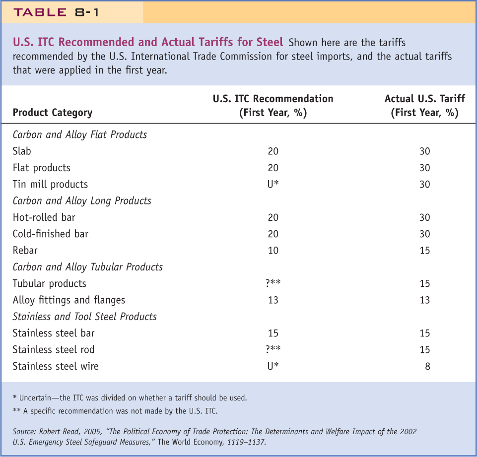
To fulfill his campaign promise to protect the steel industry, President George W. Bush requested that the ITC initiate a Section 201 investigation into the steel industry. This was one of the few times that a president had initiated a Section 201 action; usually, firms or unions in an industry apply to the ITC for import protection. After investigating, the ITC determined that the conditions of Section 201 and Article XIX were met and recommended that tariffs be put in place to protect the U.S. steel industry. The tariffs recommended by the ITC varied across products, ranging from 10% to 20% for the first year, as shown in Table 8-1, and then falling over time so as to be eliminated after three years.
249
The ITC decision was based on several factors.7 First, imports had been rising and prices were falling in the steel industry from 1998 to early 2001, leading to substantial losses for U.S. firms. Those losses, along with falling investment and employment, met the condition of “serious injury.” An explanation given by the ITC for the falling import prices was that the U.S. dollar appreciated substantially prior to 2001: as the dollar rises in value, foreign currencies become cheaper and so do imported products such as steel, as occurred during this period. To meet the criterion of Section 201 and Article XIX, rising imports need to be a “substantial cause” of serious injury, which is defined as “a cause which is important and not less than any other cause.” Sometimes another cause of injury to U.S. firms can be a domestic recession, but that was not the case in the years preceding 2001, when demand for steel products was rising.8
President Bush accepted the recommendation of the ITC but applied even higher tariffs, ranging from 8% to 30%, as shown in Table 8-1, with 30% tariffs applied to the most commonly used steel products (such as flat-rolled steel sheets and steel slab). Initially, the tariffs were meant to be in place for three years and to decline over time. Knowing that U.S. trading partners would be upset by this action, President Bush exempted some countries from the tariffs on steel. The countries exempted included Canada, Mexico, Jordan, and Israel, all of which have free-trade agreements with the United States, and 100 small developing countries that were exporting only a very small amount of steel to the United States.
250
Use this as an excuse to work through another numerical example--drawing the graph and using these numbers.
Deadweight Loss Due to the Steel Tariff To measure the deadweight loss due to the tariffs levied on steel, we need to estimate the area of the triangle b + d in Figure 8-5(b). The base of this triangle is the change in imports due to the tariffs, or ΔM = M1 − M2. The height of the triangle is the increase in the domestic price due to the tariff, or ΔP = t. So the deadweight loss equals

It is convenient to measure the deadweight loss relative to the value of imports, which is PW · M. We will also use the percentage tariff, which is t/PW, and the percentage change in the quantity of imports, which is %ΔM = ΔM/M. The deadweight loss relative to the value of imports can then be rewritten as
For the tariffs on steel, the most commonly used products had a tariff of 30%, so that is the percentage increase in the price: t/PW = 0.3. It turns out that the quantity of steel imports also fell by 30% the first year after the tariff was imposed, so that %ΔM = 0.3. Therefore, the deadweight loss is

The value of steel imports that were affected by the tariff was about $4.7 billion in the year prior to March 2002 and $3.5 billion in the year after March 2002, so average imports over the two years were  (4.7 + 3.5) = $4.1 billion (these values do not include the tariffs).9
If we apply the deadweight loss of 4.5% to the average import value of $4.1 billion, then the dollar magnitude of deadweight loss is 0.045 · 4.1 billion = $185 million. As we discussed earlier, this deadweight loss reflects the net annual loss to the United States from applying the tariff. If you are a steelworker, then you might think that the price of $185 million is money well spent to protect your job, at least temporarily. On the other hand, if you are a consumer of steel, then you will probably object to the higher prices and deadweight loss. In fact, many of the U.S. firms that purchase steel—such as firms producing automobiles—objected to the tariffs and encouraged President Bush to end them early. But the biggest objections to the tariffs came from exporting countries whose firms were affected by the tariffs, especially the European countries.
251
Response of the European Countries The tariffs on steel most heavily affected Europe, Japan, and South Korea, along with some developing countries (Brazil, India, Turkey, Moldova, Romania, Thailand, and Venezuela) that were exporting a significant amount of steel to the United States. These countries objected to the restriction on their ability to sell steel to the United States.
The countries in the European Union (EU) therefore took action by bringing the case to the WTO. They were joined by Brazil, China, Japan, South Korea, New Zealand, Norway, and Switzerland. The WTO has a formal dispute settlement procedure under which countries that believe that the WTO rules have not been followed can bring their complaint and have it evaluated. The WTO evaluated this case and, in early November 2003, ruled that the United States had failed to sufficiently prove that its steel industry had been harmed by a sudden increase in imports and therefore did not have the right to impose “safeguard” tariffs.
The WTO ruling was made on legal grounds: that the United States had essentially failed to prove its case (i.e., its eligibility for Article XIX protection).10 But there are also economic grounds for doubting the wisdom of the safeguard tariffs in the first place. Even if we accept that there might be an argument on equity or fairness grounds for temporarily protecting an industry facing import competition, it is hard to argue that such protection should occur because of a change in exchange rates. The U.S. dollar appreciated for much of the 1990s, including the period before 2001 on which the ITC focused, leading to much lower prices for imported steel. But the appreciation of the dollar also lowered the prices for all other import products, so many other industries in the United States faced import competition, too. On fairness grounds, there is no special reason to single out the steel industry for protection.
The WTO ruling entitled the European Union and other countries to retaliate against the United States by imposing tariffs of their own against U.S. exports. The European countries quickly began to draw up a list of products—totaling some $2.2 billion in U.S. exports—against which they would apply tariffs. The European countries naturally picked products that would have the greatest negative impact on the United States, such as oranges from Florida, where Jeb Bush, the president’s brother, was governor.
The threat of tariffs being imposed on these products led President Bush to reconsider the U.S. tariffs on steel. On December 5, 2003, he announced that they would be suspended after being in place for only 19 months rather than the three years as initially planned. This chain of events illustrates how the use of tariffs by an importer can easily lead to a response by exporters and a tariff war. The elimination of the steel tariffs by President Bush avoided such a retaliatory tariff war.
Tariff on Tires The tariff on tires imported from China, announced by President Obama on September 11, 2009, was requested by the United Steel, Paper and Forestry, Rubber, Manufacturing, Energy, Allied Industrial, and Service Workers International Union (or the United Steelworkers, for short), the union that represents American tire workers. On April 20, 2009, they filed a petition with the U.S. ITC for import relief under Section 421 of U.S. trade law. As discussed in Side Bar: Safeguard Tariffs, this section of U.S. trade law enables tariffs to be applied against products imported from China if the imports are “a significant cause of material injury” to the U.S. industry. A majority of the ITC commissioners felt that rising imports from China of tires for cars and light trucks fit this description and recommended that tariffs be applied for a three-year period. Their recommendation was for tariffs of 55% in the first year, 45% in the second year, and 35% in the third year (these tariffs would be in addition to a 4% tariff already applied to U.S. tire imports).
252
President Obama decided to accept this recommendation from the ITC, which was the first time that a U.S. President accepted a tariff recommendation under Section 421. From 2000 to 2009, there had been six other ITC investigations under Section 421, and in four of these cases a majority of commissioners voted in favor of tariffs. But President George W. Bush declined to apply tariffs in all these cases. In accepting the recommendation to apply tariffs on tires, however, President Obama reduced the amount of the tariff to 35% in the first year starting September 26, 2009, 30% in the second year, and 25% in the third year, with the tariff expiring on September 27, 2012.
We’ve already noted one key difference between the tariff on tires and the earlier tariff on steel: the tire tariff was applied to imports from a single country—China—under Section 421 of U.S. trade law, whereas the steel tariff was applied against many countries under Section 201. For this reason we will refer to the tariff on tires applied against China as a discriminatory tariff, meaning a tariff that is applied to the imports from a specific country. Notice that a discriminatory tariff violates the “most favored nation” principle of the WTO and GATT (see Sidebar: Key Provisions of the GATT), which states that all members of the WTO should be treated equally. It was possible for the United States to apply this discriminatory tariff against China because Section 421 was negotiated as a condition for China entering the WTO.
Discuss who might have supported it. Unions?
A second difference between these cases is that steel producers in the United States supported that tariff, but no U.S. tire producers joined in the request for the tariff on tires. There are 10 producers of tires in the United States, and seven of them—including well-known firms like Goodyear, Michelin, Cooper, and Bridgestone—also produce tires in China and other countries. These firms naturally did not want the tariff put in place because it would harm rather than help them.
There are also a number of similarities in the two cases. As occurred in steel, the tariff on tires led to retaliation. China responded with actual or potential tariffs on products such as chicken feet (a local delicacy), auto parts, certain nylon products, and even passenger cars. For its part, the United States went on to apply new tariffs on steel pipe imported from China, and also investigated several other products. Another similarity with the steel case is that China made an official complaint to the WTO under its dispute settlement procedure, just as the European countries did in the steel case. China claimed that the “significant cause of material injury” conditions of Section 421 had not been met. China also questioned whether it was legal under the WTO for the United States to apply a discriminatory tariff. Unlike the steel case, the WTO concluded that the United States was justified in applying the tariff on tires.
The final comparison we make between the steel and tire tariffs focuses on the calculation of the deadweight losses. Because the tariff on tires was applied against only one country—China—you might think that it would have a lower deadweight loss that the steel tariff, which was applied against many countries selling to the United States. It turns out that the opposite is true: the tariff on tires had a higher deadweight loss than that tariff on steel, precisely because it was a discriminatory tariff that was applied against only one country. To explain this surprising outcome, we will make use of Figure 8-6.
253
An important principle, but don't rush through the proof.
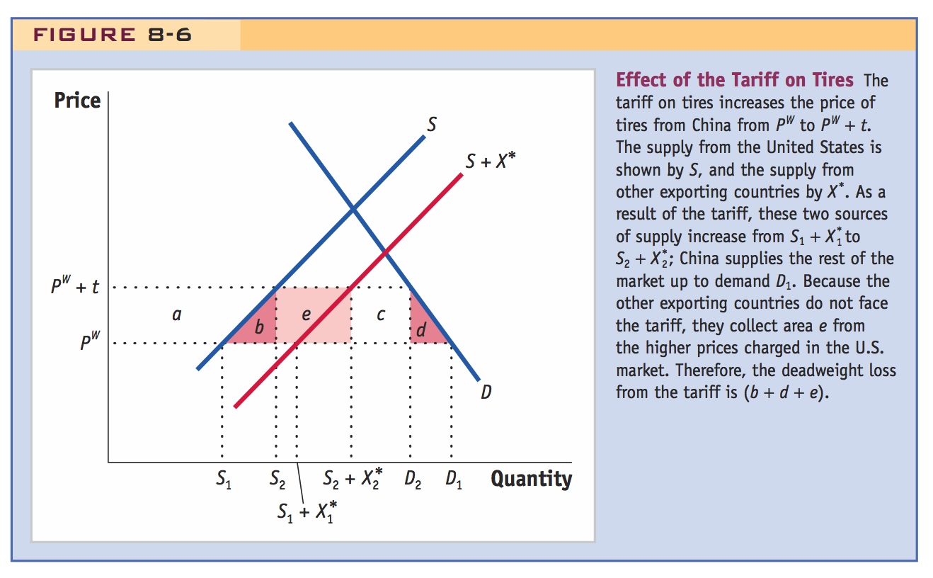
A Discriminatory Tariff We suppose that China can sell any amount of tires to the United States at the price of PW in Figure 8-6. What is new in this figure is the treatment of the other countries exporting to the United States. We represent these countries by the upward-sloping supply curve X*, which is added onto U.S. supply of S to obtain total supply from all countries other than China of S + X*.
Under free trade, the price for tires is PW and the supply from the United States is S1. Supply from the United States and exporting countries other than China is S1 +  , while China exports the difference between S1 + and demand of D1. When the tariff of t is applied against China, the price of tires rises to PW + t, supply from the United States rises to S2. Supply from the United States and exporting countries other than China rises to S2 +
  . China exports the difference between S2 + and demand of D2. Because the price has risen to PW + t, both U.S. producers and exporting countries other than China are selling more (moving along their supply curves) while China must be selling less (because the other countries are selling more and total demand has gone down).
So far the diagram looks only a bit different from our treatment of the tariff in Figure 8-5. But when we calculate the effect of the tariff on welfare in the United States, we find a new result. We will not go through each of the steps in calculating the change in consumer and producer surplus, but will focus on tariff revenue and the difference with our earlier treatment in Figure 8-5. The key idea to keep in mind is that the tariff applies only to China, and not to other exporting countries. So with the increase in the price of tires from PW to PW + t, the other exporting countries get to keep that higher price: it is not collected from these countries as tariff revenue. Under these circumstances, the amount of tariff revenue is only the quantity that China exports (the difference between S2 + and demand of D2) times the tariff t, which is the area shown by c. In comparison, the area shown by e is the increase in the price charged by other exporters times their exports of . Area e is not collected by the U.S. government as tariff revenue, and becomes part of the deadweight loss for the United States. The total deadweight loss for the U.S. is then (b + d + e), which exceeds the deadweight loss of (b + d) that we found in Figure 8-5. The reason that the deadweight loss has gone up is that other exporters are selling for a higher price in the United States, and the government does not collect any tariff revenue from them.
254
Deadweight Loss Due to the Tire Tariff Figure 8-6 shows that a discriminatory tariff applied against just one country has a higher deadweight loss, of (b + d + e), than an equal tariff applied against all exporting countries, in which case the deadweight loss is just (b + d) as we found in Figure 8-5. To see whether this theoretical result holds in practice, we can compare the tariff on tires with the tariff on steel. In the end, we will find that the tariff on tires was costlier to the United States because other countries—especially Mexico and other countries from Asia—were able to sell more tires to the United States at higher prices.
The effect of the tariff on the percentage of U.S. import value coming from China and other countries is shown in Figure 8-7. Just before the tariff was imposed in September 2009, imports into the United States were evenly divided with one-third coming from China, one-third from other Asian countries, and one-third from Canada, Mexico, and all other countries. The lowest area in the graph represents the value of imports from China. We can see that Chinese imports dropped in the fourth quarter (Q4) of 2009, after the tariff began in September, and rose again in the fourth quarter (Q4) of 2012, after the tariff ended in September of that year. The value of imports from China fell from about 33% of overall imports to 15% when the tariff began, and rose from about 12% of overall imports to 22% after the tariff ended. But this 18 percentage point decline in imports from China when the tariff began was substantially made up by increased imports from other Asian countries. We can see this result by looking at the next area shown in the graph, above China, which represents imports from all other Asian countries. When adding up the Chinese and other Asian imports, we obtain about 60% of the total imports, and while this percentage varies to some extent when the tariff begins and ends, it varies much less than does the percentage imported from China itself. In other words, other Asian countries made up for the reduction in China exports by increasing their own exports; similarly, Mexico (included within the top area in the graph) also increased its exports to the United States during the time the tariff was applied.
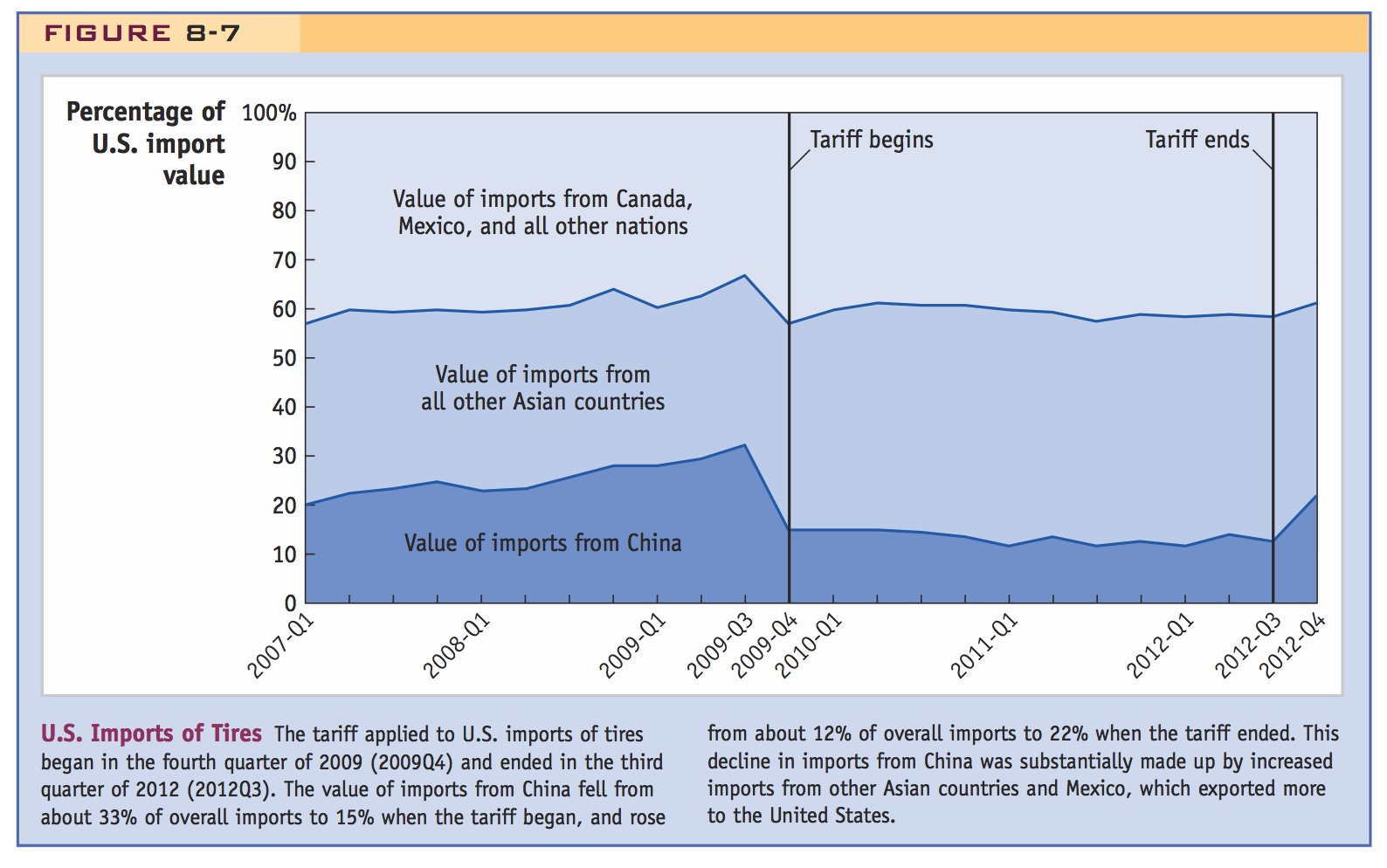
This increase in sales from other Asian countries and Mexico is consistent with Figure 8-6, which shows that sales from other exporters increase from to due to the tariff on China. The evidence also indicates that these other exporters were able to charge higher prices for the tires they sold to the United States. For car tires, the average price charged by countries other than China increased from $54 to $64 during the times of the tariff, while for light truck tires, the average prices increased from $76 to $90. Both these increases are higher than we would expect from inflation during 2009–12. As shown in Figure 8-6, these price increases for other exporters occur because they are competing with Chinese exporters who must pay the tariff.
255
Hufbauer has a lot of accessible work estimating the costs of protectionist policies (and at least one book) that could be assigned as outside reading or case studies.
An estimate of the area e—which is the total increase in the amount paid to tire exporters other than China—is $716 million per year for imports of car tires and another $101 million per year for imports of light truck tires, totaling $817 million per year.11 This is in addition to the deadweight loss (b + d). This area e for the tire tariff substantially exceeds the deadweight loss for the steel tariff of $185 million per year that we calculated above. So we see that a discriminatory tariff, applied against just one exporting country, can be more costly then an equal tariff applied against all exporters.
At the beginning of the chapter we included a quote from President Obama in his State of the Union address in 2012, in which he said that “over a thousand Americans are working today because we stopped a surge in Chinese tires.” Although 1,000 jobs in the tire industry is roughly the estimate of how many jobs were saved, we have shown that these jobs came at a very high cost because the tariff was discriminatory.12 In a later chapter we will discuss another example like this which shows that opening up free trade with just one country can have a surprising negative effect on welfare as compared with opening up free trade with all countries.
256