module 22 Human Population Numbers
Although it may seem surprising, environmental scientists do not know the human carrying capacity of Earth. However, we are able to discuss the factors that contribute to the carrying capacity of humans on Earth and what drives human population growth. We can also look at patterns of past human population growth to gain an understanding of what might occur in future decades.
Learning Objectives
After reading this module you should be able to
explain factors that may potentially limit the carrying capacity of humans on Earth.
describe the drivers of human population growth.
read and interpret an age structure diagram.
Scientists disagree on Earth’s carrying capacity
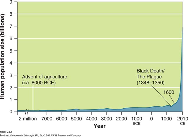
Every 5 days, the global human population increases by more than a million lives: 1.9 million infants are born and 800,000 people die. The human population has not always grown at this rate, however. As FIGURE 22.1 shows, until a few hundred years ago the human population was relatively stable: Deaths and births occurred in roughly equal numbers. This situation changed about 400 years ago, when agricultural output increased and sanitation began to improve. Better living conditions caused death rates to fall, but birth rates remained relatively high. This was the beginning of a period of rapid population growth that has brought us to the current human population of 7.2 billion people.
As we saw in Chapter 6, under ideal conditions all populations grow exponentially. In most cases, exponential growth slows or stops when an environmental limit is reached. The limiting factor can be a scarcity of resources such as food or water or an increase in predators, parasites, or diseases. Limiting factors determine the carrying capacity of a habitat. Are human populations constrained by limiting factors?
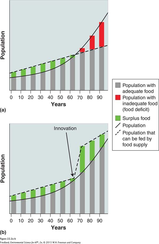
Environmental scientists have differing opinions on Earth’s carrying capacity for humans. Some scientists believe we have already outgrown, or eventually will outgrow, the available supply of food, water, timber, fuel, and other resources on which humans rely. One of the first proponents of the notion that the human population could exceed Earth’s carrying capacity was English clergyman and professor Thomas Malthus. In 1798, Malthus observed that the human population was growing exponentially while the food supply we rely on was growing linearly. In other words, the food supply increases by a fixed amount each year, while the human population increases in proportion to its own increasing size. Malthus concluded that the human population size would eventually exceed the food supply. FIGURE 22.2a shows this projection graphically.
A number of environmental scientists today subscribe to Malthus’s view that humans will eventually reach the carrying capacity of Earth, after which the rate of population growth will decline. Other scientists do not believe that Earth has a fixed carrying capacity for humans. They argue that the growing population of humans provides an increasing supply of intellect that leads to increasing amounts of innovation. Humans can alter Earth’s carrying capacity by employing creativity—
For example, in the past whenever the food supply seemed small enough to limit the human population, major technological advances increased food production. This progression began thousands of years ago. The development of arrows made hunting more efficient, which allowed hunters to feed a larger number of people. Early farmers increased crop yields with hand plows and later with oxen-
The ability of humans to innovate in the face of challenges has led some scientists to expect that we will continue to make technological advances indefinitely. This expectation is reasonable, but questions remain. Based on our history, should we assume that humans will continue to find ways to feed a growing population? Are there other limits to human population growth? And how do we know if we have exceeded Earth’s carrying capacity?
Many factors drive human population growth
Demography The study of human populations and population trends.
Demographer A scientist in the field of demography.
As we know from our study of biological populations, a variety of factors influence the growth, reproduction, and success of plant and animal species. Many of these same factors influence human populations as well. Population size, birth and death rates, fertility, life expectancy, and migration are factors that influence population size in countries. In order to understand the impact of the human population on the environment, we must first understand what drives human population growth. The study of human populations and population trends is called demography, and scientists in this field are called demographers. By analyzing specific data such as changes in population size, fertility, life expectancy, and migration, demographers can offer insights—
Changes in Population Size
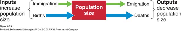
We can view the human population as a system with inputs and outputs, like all biological systems. If there are more births than deaths, the inputs are greater than the outputs, and the system expands. For most of human history, total births slightly outnumbered total deaths, resulting in very slow population growth. If the reverse had been true, the human population would have decreased and would have eventually become extinct.
Immigration The movement of people into a country or region, from another country or region.
Emigration The movement of people out of a country or region.
When demographers look at population trends in individual countries, they take into account inputs and outputs. As FIGURE 22.3 shows, inputs include both births and immigration, which is the movement of people into a country or region from another country or region. Outputs, or decreases, include deaths and emigration, which is the movement of people out of a country or region. When inputs to the population are greater than outputs, the growth rate is positive. Conversely, if outputs are greater than inputs, the growth rate is negative.
Crude birth rate (CBR) The number of births per 1,000 individuals per year.
Crude death rate (CDR) The number of deaths per 1,000 individuals per year.
Demographers use specific measurements to determine yearly birth and death rates. The crude birth rate (CBR) is the number of births per 1,000 individuals per year. The crude death rate (CDR) is the number of deaths per 1,000 individuals per year. Worldwide, there were 20 births and 8 deaths per 1,000 people in 2014. We do not factor in migration for the global population because, even though people move from place to place, they do not leave Earth. Thus, in 2014, the global population increased by 12 people per 1,000 people. This rate can be expressed mathematically as a percentage:
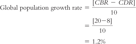
We divide by 10 to arrive at the percentage because the birth and death rates are expressed per 1,000 people.
To calculate the population growth rate for a single nation, we take immigration and emigration into account:

Doubling time The number of years it takes a population to double.
If we know the growth rate of a population and assume that growth rate is constant, we can calculate the number of years it takes for a population to double, which is known as its doubling time. As a population grows rapidly, the doubling time gives us a better sense of the magnitude of the change than the growth rate alone. Because growth rates may change in future years, we can never determine a country’s doubling time with certainty. Therefore, we say that a population will double in a certain number of years if the growth rate remains constant.
The doubling time can be approximated mathematically using a formula called the rule of 70:
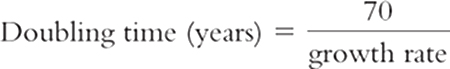
Therefore, a population growing at 2 percent per year will double every 35 years:
Note that this is true of any population growing at 2 percent per year, regardless of the size of that population. At a 2 percent growth rate, a population of 50,000 people will increase by 50,000 in 35 years, and a population of 50 million people will increase by 50 million in 35 years.
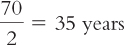
As we saw in FIGURE 22.1, Earth’s population has doubled several times since 1600. It is almost certain, however, that Earth’s population will not double again. FIGURE 22.4 shows the current projections through the year 2100. Most demographers believe that the human population will be somewhere between 8.1 billion and 9.6 billion in 2050 and will stabilize between 6.8 billion and 10.5 billion by roughly 2100.
Fertility
Total fertility rate (TFR) An estimate of the average number of children that each woman in a population will bear throughout her childbearing years.
To understand more about the role births play in population growth, demographers look at the total fertility rate (TFR), an estimate of the average number of children that each woman in a population will bear throughout her childbearing years (between the onset of puberty and menopause). For example, in the United States in 2014, the TFR was 1.9, meaning that, on average, each woman of childbearing age gave birth to just under 2 children. Note that, unlike crude birth rate and crude death rate, TFR is not calculated per 1,000 people. Instead, it is a measure of births per woman.
Replacement-
To gauge changes in population size, demographers also calculate replacement-
Developed country A country with relatively high levels of industrialization and income.
Developing country A country with relatively low levels of industrialization and income.
In developed countries—countries with relatively high levels of industrialization and income—
In a country where TFR is equal to replacement-
Life Expectancy
Life expectancy The average number of years that an infant born in a particular year in a particular country can be expected to live, given the current average life span and death rate in that country.
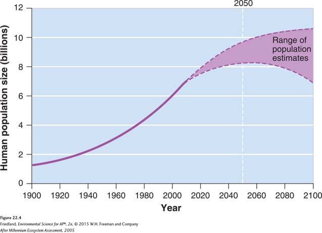
To understand more about the outputs in a human population system, demographers study the human life span. Life expectancy is the average number of years that an infant born in a particular year in a particular country can be expected to live, given the current average life span and death rate in that country. Life expectancy is generally higher in countries with better health care. A high life expectancy also tends to be a good predictor of high resource consumption rates and environmental impacts. FIGURE 22.5 shows life expectancies around the world.
Life expectancy is often reported in three different ways: for the overall population of a country, for males only, and for females only. For example, in 2014, global life expectancy was 70 years overall, 68 years for men, and 72 years for women. In the United States, life expectancy was 76 years overall, 73 years for men, and 81 years for women. In general, human males have higher death rates than human females, leading to a shorter life expectancy for men. In addition to biological factors, men have historically tended to face greater dangers in the workplace, made more hazardous lifestyle choices, and been more likely to die in wars. Cultures have changed over time, however, and as more and more women enter the workforce and the armed forces, the life expectancy gap between men and women will probably decrease.
Infant and Child Mortality
Infant mortality The number of deaths of children under 1 year of age per 1,000 live births.
Child mortality The number of deaths of children under age 5 per 1,000 live births.
The availability of health care, access to good nutrition, and exposure to pollutants are all factors in life expectancy, infant mortality, and child mortality. The infant mortality rate is defined as the number of deaths of children under 1 year of age per 1,000 live births. The child mortality rate is defined as the number of deaths of children under age 5 per 1,000 live births. FIGURE 22.6 shows infant mortality rates around the world.
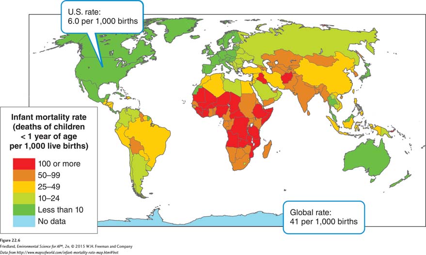
If a country’s life expectancy is relatively high and its infant mortality rate is relatively low, it is likely that the country has a high level of available health care, an adequate food supply, potable drinking water, good sanitation, and a moderate level of pollution. Conversely, if its life expectancy is relatively low and its infant mortality rate is relatively high, it is likely that the country’s population does not have sufficient health care or sanitation and that potable drinking water and food are in limited supply. Pollution and exposure to other environmental hazards may also be high. In 2014, the global infant mortality rate was 41. In the United States, the infant mortality rate was 5.9. In other developed countries, such as Sweden (2.6) and France (3.3), the infant mortality rate was even lower. Availability of prenatal care is an important predictor of the infant mortality rate. For example, the infant mortality rate is 63 in Liberia and 40 in Bolivia, both countries where many women do not have good access to prenatal care.
Sometimes, life expectancy and infant mortality in a given sector of a country’s population differ widely from life expectancy and infant mortality in the country as a whole. In this case, even when the overall numbers seem to indicate a high level of health care throughout the country, the reality may be starkly different for a portion of its population. For example, whereas the infant mortality rate for the U.S. population as a whole is 6.0, it is 12.4 for African Americans, 8.5 for Native Americans, and 5.3 for Caucasians. This variation in infant mortality rates is probably related to socioeconomic status and varying degrees of access to adequate nutrition and health care. These differences are often issues of environmental justice, a topic we discuss in more detail in Chapter 20.
Aging and Disease
Even with a high life expectancy and a low infant mortality rate, a country may have a high crude death rate, in part because it has a large number of older individuals. The United States, for example, has a higher standard of living than Mexico, which is consistent with the higher life expectancy and lower infant mortality rate in the United States. At the same time, the United States has a much higher CDR, at 8 deaths per 1,000 people on average, than Mexico, which has 5 deaths per 1,000 people on average. This higher CDR results from the much larger elderly population in the United States, with 13 percent of its population aged 65 years or older, compared with the 6 percent of the population aged 65 or older in Mexico.
Disease is an important regulator of human populations. According to the World Health Organization, infectious diseases—
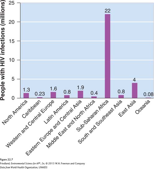
HIV has a significant effect on infant mortality, child mortality, population growth, and life expectancy. In Lesotho, in southern Africa, where 23 percent of the adult population is infected with HIV, life expectancy fell from 63 years in 1995 to 40 years in 2009. It has since been increasing and is now approximately 48.
As FIGURE 22.7 shows, approximately 34 million people were living with HIV in 2011, 22 million of them in sub-
Migration
Net migration rate The difference between immigration and emigration in a given year per 1,000 people in a country.
Regardless of its birth and death rates, a country may experience population growth, stability, or decline as a result of migration. Net migration rate is the difference between immigration and emigration in a given year per 1,000 people in a country. A positive net migration rate means there is more immigration than emigration, and a negative net migration rate means the opposite. For example, approximately 1 million people immigrate to the United States each year, and only a small number emigrate. With a U.S. population of 315 million, these rates are equal to 3.2 immigrants per 1,000 people.
A country with a relatively low CBR but a high immigration rate may still experience population growth. For example, the United States has a TFR of 1.9, but it has a high net migration. As a result, the U.S. population will probably increase by 30 percent by 2050. Canada has a net migration rate of 0.7 per 1,000 and a TFR of 1.6, which is well below replacement-
In countries with a negative net migration rate and a low TFR, the population actually decreases over time. Very few countries fit this model. One is the country of Georgia, in western Asia. It has a growth rate of 0.2 percent, a TFR of 1.7, and a net migration rate of –5 per 1,000. Georgia is projected to have a 20 percent population decrease by 2050.
We have noted that although the movement of people around the world does not affect the total number of people on the planet, migration is still an important issue in environmental science. The movement of people displaced because of disease, natural disasters, environmental problems, or conflict can create crowded, unsanitary conditions, and shortages of food and water. In some cases people are moved into refugee camps where they have little opportunity to improve their conditions through employment or emigration. All of these situations can easily become humanitarian and environmental health issues. The movement of people from developing countries to developed countries tends to increase the ecological footprint of those people because, over time, immigrants typically adopt the lifestyle and consumption habits of their new country. A person who migrates from Mexico to the United States, for example, is likely to use more resources as a U.S. resident than as a resident of Mexico because the United States typically has a more affluent lifestyle.
Age structure diagrams describe how populations are distributed across age ranges
Age structure diagram A visual representation of the number of individuals within specific age groups for a country, typically expressed for males and females.
Demographers use data on age to predict how rapidly a population will increase and what its size will be in the future. The age structure of a population describes how its members are distributed across age ranges, usually in 5-
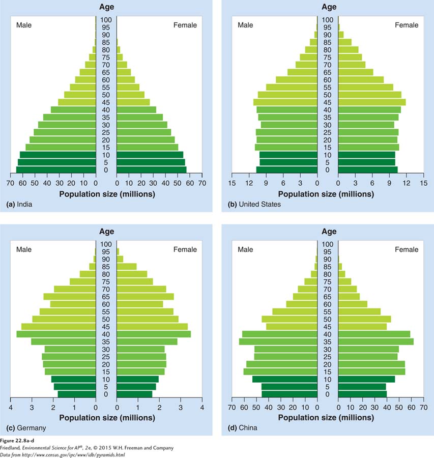
Population pyramid An age structure diagram that is widest at the bottom and smallest at the top, typical of developing countries.
While every nation has a unique age structure, we can group countries very broadly into three categories. A country with many more younger people than older people has an age structure diagram that is widest at the bottom and narrowest at the top, as shown in FIGURE 22.8a. This type of age structure diagram, called a population pyramid, is typical of developing countries, such as Venezuela and India. The wide base of the graph compared with the levels above it indicates that the population will grow because a large number of females aged 0 to 15 have yet to bear children. Even if each one of these future potential mothers has only two children, the population will grow simply because there are increasing numbers of women able to give birth.
Population momentum Continued population growth after growth reduction measures have been implemented.
The population pyramid can also be used to illustrate how long a time it takes for changes to affect a growing population. Population momentum is continued population growth after growth reduction measures have been implemented. It occurs because there are relatively large numbers of individuals at reproductive maturity in the population. Population momentum has been compared with the momentum of a long, heavy freight train, which takes longer to stop than a shorter, lighter freight train. It is the reason why a population keeps on growing after birth control policies or voluntary birth reductions have begun to lower the CBR of a country. Eventually, over several generations, those actions will bring the population to a more stable growth rate but the momentum of all the individuals who have recently reached child-
A country with little difference between the number of individuals in younger age groups and in older age groups has an age structure diagram that looks more like a column from age 0 through age 50, as shown in FIGURE 22.8b. If a country has few individuals in the younger age classes, we can deduce that it has slow population growth or is approaching no growth at all. The United States, Canada, Australia, Sweden, and many other developed countries have this type of age structure diagram. A number of developing countries that have recently lowered their growth rates should begin to show this pattern within the next 10 to 15 years.
A country with a greater number of older people than younger people has an age structure diagram that resembles an inverted pyramid. Such a country has a total fertility rate below 2.1 and a decreasing number of females within each younger age range. Such a population will continue to shrink. Italy, Germany, Russia, and a few other developed countries display this pattern, seen in Figures 22.8c and 22.8d. China is in the very early stages of showing this pattern.