In the models we’ve studied so far, we haven’t considered the possibility that other firms might want to enter markets in which firms are earning positive economic profits. Presumably, other firms exist that would like a piece of that action. If there are no barriers to entering a market such as the snowboard market, an additional firm will cause Burton and K2’s profits to decline. We saw in the Cournot model that adding more firms to the industry drove the equilibrium closer to perfect competition. In this section, we look at our last model of imperfect competition, and see what happens when there is entry into a market with differentiated products. Monopolistic competition is a market structure characterized by many firms selling a differentiated product with no barriers to entry. This term might sound like an oxymoron—competitive monopoly?—and in a way it is, but the term reflects the basic tension between market power and competitive forces that exists in these types of markets.

454

Every firm in a monopolistically competitive industry faces a downward-sloping demand curve, so it has some market power and every firm follows the monopoly pricing rule. That’s where the “monopolistic” comes from. What is competitive about such markets is that there are no restrictions on entry as exist in monopoly markets—any number of firms can come into the industry at any time. This means that the firms in a monopolistically competitive industry, despite having market power, earn zero economic profit. (If they were making a profit, more firms would enter to acquire some of this profit. Entry only stops when profit is driven to zero for every firm in the market.)

Many markets are monopolistically competitive. For example, there are hundreds of fast-food restaurants in Chicago. Some differences between them exist, but basically people view such restaurants as largely interchangeable. Because travel is costly, though, each restaurant has a bit of market power in its local neighborhood. So, a restaurant does have some ability to set its own prices. At the same time, however, there’s little to stop a new restaurant from opening. If people in a neighborhood become more enthralled with eating out, an existing restaurant might be able to raise its prices and earn economic profit for a brief period, but if the trend lasts, it is likely that a new restaurant will open up to grab some of that profit.

Keep in mind that, while monopolistic competition is categorized as “imperfect competition” along with oligopoly, there are differences between these two market structures. One is that oligopoly markets have barriers to entry, while monopolistically competitive markets do not. However, the key distinction between oligopoly and monopolistic competition is the assumption about strategic interaction. In an oligopoly, firms know that their production decisions affect their competitors’ optimal choices, and all oligopolistic firms take this feedback effect into account when making their decisions. On the other hand, in monopolistic competition, firms do not worry about the production decisions of their competitors because the impact of any competitor on another is assumed to be too small for these firms to be concerned about.

To analyze monopolistically competitive markets, let’s look at a single company with market power—say for a moment that, for some reason, a city has only one fast-food restaurant. In this city, this restaurant has a monopoly on fast food. The firm faces a downward-sloping demand curve for meals served per day, as in Figure 11.6. We’ll label this demand D_ONE (for one firm). The figure also shows the marginal revenue curve that corresponds to this demand, as well as the firm’s average total and marginal cost curves.

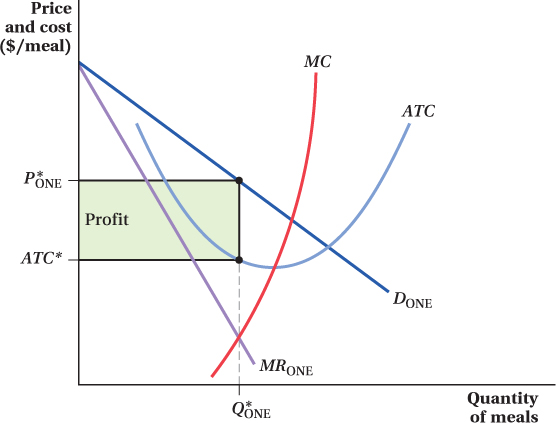
Because the restaurant in Figure 11.6 is a monopolist, it produces where its marginal revenue equals marginal cost, Q*_ONE. The price it charges is P*_ONE In addition to the marginal cost of production, however, the restaurant has to pay fixed cost equal to F (this fixed cost is the reason why the firm’s average total cost curve is U-shaped). The monopolist restaurant’s profit is shown by the shaded rectangle: the difference between the price and the average total cost at the quantity produced, multiplied by that quantity. Because average total cost includes both variable and fixed costs, the average total cost at Q*_ONE —that is, ATC*—fully reflects all the firm’s production costs.

So far, this market is just a regular monopoly. But now suppose another restaurateur notices that this firm makes economic profit and decides to open a second, slightly different fast-food restaurant in the city. The new restaurant may differ in location, type of food served, anything that differentiates it from the existing restaurant.

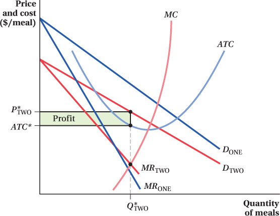
The key to understanding what happens in monopolistically competitive markets is to recognize what happens to the demand curve(s) of the market’s existing firm(s) when another firm enters. We know that when there are more substitutes for a good available, the demand curve for the initial good becomes more elastic (less steep). Having another restaurant open up means that more substitution possibilities now exist for consumers. Instead of there being one firm with a demand curve, as in Figure 11.6, the entry of a second firm means each restaurant now has a demand curve that is a bit flatter than the monopolist firm’s demand curve. And, because the demand is being split across two firms, not only is the monopolist firm’s demand curve flatter, but it has shifted in as well. Figure 11.7 shows this change from one to two firms, as the initial (monopolist) firm’s demand curve (now it is a residual demand curve) shifts from D_ONE to D_TWO . Notice how D_TWO is both flatter than D_ONE and to the left of it. The marginal revenue curves also shift accordingly. (The figure illustrates only what’s going on for one of the two firms in the market; the picture is exactly the same for the other firm.)

455

456

Even after entry, however, both firms are essentially monopolists over their own residual demand curves. Each individual firm’s demand curve reflects the fact that (1) it is splitting the market with another firm and (2) the presence of a substitute product makes the firm’s demand more elastic. The competitor’s presence is accounted for, but it is incorporated in the firm’s residual demand curve. In monopolistic competition, the firm takes this residual demand as given. This is different from the oligopoly models we covered, in which firms realize that their actions affect the desired actions of their competitors, which in turn affect their own optimal action, and so on. This strategic interaction is captured in firms’ reaction curves. A monopolistically competitive firm, on the other hand, acts like it is in its own little monopoly world, even though its competitors’ actions affect the residual demand it faces. This assumption about monopolistically competitive firms’ ignorance of strategic interactions is more likely to hold in industries where there are a large number of firms selling related but differentiated products such as car washes, self-storage, and mattress stores.

Assuming the two firms have identical residual demand curves, both produce the quantity Q*_TWO at which marginal revenue equals marginal cost and charge the profit-maximizing price P*_TWO at that quantity. Each firm earns the profit given by the shaded rectangle in the figure.

Because two firms in the market make positive economic profit, still more firms will want to enter. Each new firm that enters will further shift the other individual companies’ demand curves to the left and make them more elastic (flatter).

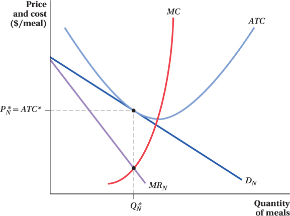
Entry will cease only when industry firms are no longer making economic profit. At that point, the market will look like Figure 11.8. When there are N firms in the market, each firm’s residual demand curve eventually shifts back to D_N . Faced with this demand curve, the firm produces the quantity Q*_N at which marginal revenue equals marginal cost, charges a price of P*_N , and earns zero economic profit.

457

Why does economic profit equal zero at this point? Look at where the firm’s average total cost curve is relative to its demand curve. The two curves are tangent at Q*_N and P*_N. If price equals average total cost, profit is zero. The firm is just covering its costs of operation (variable and fixed) at this point.

Here’s an important point about monopolistically competitive markets: Even though entry occurs until profits are zero, the entry process does not ultimately lead to a perfectly competitive outcome in which price equals marginal cost. Firms in a monopolistically competitive market face a downward-sloping demand curve, so marginal revenue is always less than price. At the profit-maximizing output, marginal cost will equal marginal revenue, which means that marginal cost will also be less than price. Free entry ensures that this markup over marginal cost is just enough to cover the firm’s fixed cost, and no more.