We start our analysis of factor markets by looking at the market for labor inputs. The labor market is probably the most important factor market. In most economies, about 60–70% of the money spent on inputs is paid to workers. Once we understand how the labor market works, the analysis of any factor market follows the same pattern.

The demand side of the labor market comprises all firms that would like to hire workers to make outputs. We begin by looking at a single firm’s demand for labor. After that, we add up such demands across all firms to obtain the total market demand for labor.

512

Let’s think about a company (say, Samsung) that needs to buy (or hire) labor to produce an output (smartphones). As with our analysis of other markets, we make some simplifying assumptions so that we can boil down complex market interactions to something we can get a grip on, while not simplifying so much that we are unable to explain what’s happening.

To make our analysis simpler, we assume all labor units are the same: An employee-hour is an employee-hour, no matter who that employee is, what he does at work, or what his wage is. For now, we won’t worry about these differences, and we just say that Samsung buys “labor” at a single wage.

Another simplifying assumption we make is that Samsung chooses the short-run amount of labor to hire. Because we are looking at the short run, Samsung’s capital inputs are fixed (see Chapter 6). The firm therefore wants to hire the optimal amount of labor to work with its fixed amount of capital. Later in this chapter, we study long-run labor demand, which describes hiring when firms can also change their capital inputs.

To start to figure out Samsung’s demand for labor, think about the tradeoffs Samsung faces when it hires more labor. Adding more workers (or having its existing workers work more hours) allows Samsung to make more smartphones. The amount of additional production from a 1-unit increase in labor is the marginal product of labor, MP_L. In our example, the MP_L is the extra number of smartphones Samsung can make with one additional unit of labor. Samsung doesn’t just want to make smartphones, though; it needs to sell them. The extra revenue that those additional smartphones yield when they are sold is their marginal revenue, MR. Therefore, the total benefit to Samsung of hiring one more unit of labor is the number of phones that worker makes times the revenue earned by selling the phones—that is, the marginal product of labor times the marginal revenue. This value is called the marginal revenue product of labor, or MRP_L. Thus, MRP_L = MP_L × MR.

Samsung’s cost of hiring that additional unit of labor is the market-given wage. In a perfectly competitive market, the firm can hire as much labor as it would like at the market wage W.

Consider how this benefit (the MRP_L) and cost (W) change with the amount of labor Samsung hires. We know the cost W is fixed and thus unaffected by the amount of labor hired. On the other hand, as we learned in Chapter 6, a firm’s production exhibits diminishing marginal returns to labor and capital. Thus, labor’s marginal revenue product falls as Samsung hires more workers. The marginal product of labor MP_L goes down as a firm hires more labor because of diminishing returns (remember, capital inputs are fixed in the short run, so more and more people are using the same amount of capital). If the output market is perfectly competitive, we know from Chapter 8 that MR is constant and equal to the market price of the product. In this case, since MR is constant but MP_L falls as more labor is hired, MRP_L must drop. If instead the firm has some market power (as Samsung does in smartphones), we know from Chapter 9 that marginal revenue falls as output rises. Because more labor must be hired to produce more output, MR will fall. This drop in MR reinforces the negative effect on MP_L of hiring more labor, further causing MRP_L to fall when more labor is hired.

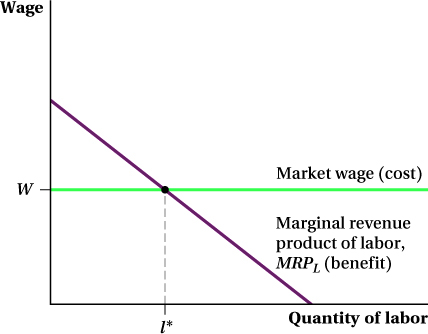
The changes in labor’s marginal revenue product as hiring changes are shown in Figure 13.1. Samsung’s marginal revenue product curve MRP_L (measured in dollars) falls as it hires more labor, and the wage it pays to the extra workers stays constant.

We now have all the elements we need to describe Samsung’s demand for labor. Think about Samsung’s tradeoff between its benefit (MRP_L) and cost (W) of hiring more labor. At relatively low levels of hiring, labor’s marginal revenue product is high because MP_L is still large. As a result, MRP_L > W. Samsung wants to hire any unit of labor for which this is true because that labor unit’s benefit is greater than its cost. In Figure 13.1, this is true for all quantities of labor less than l*.

513

Samsung will not want to hire any unit of labor for which MRP_L < W, as is the case for labor levels above l*, because the benefit of those additional units of labor MRP_L is less than their cost W.

In fact, Samsung wants to hire exactly l*. Hiring less labor would mean it isn’t employing workers whose benefit exceeds their cost. Hiring more labor than l* would mean Samsung is employing labor with a benefit below its cost. The relationship between the marginal revenue product and the wage at l* is key because it reflects what must be true at the optimal level of hiring: A firm is employing the optimal amount of labor when the marginal revenue product of labor equals the wage:

MRP_L = W

What does this optimality condition tell us about labor demand? Any demand curve shows the quantity demanded of a good as its price changes. Here, the good is labor and the price is the wage. We just saw that the MRP_L curve gives the quantity demanded at each price. If the wage changes, the amount of hiring the firm wants to do changes with it. You can see this in Figure 13.2. If the market-determined wage rises from W to W₁, fewer units of labor have a marginal revenue product that is greater than the wage, so Samsung hires only l*₁, where MRP_L = W₁. If the wage falls to W₂, Samsung hires l*₂, where MRP_L = W₂. Samsung wants to hire the quantity of labor such that the marginal revenue product of labor equals the wage. In other words, the MRP_L curve is Samsung’s labor demand curve. Like the other demand curves we’ve seen, it slopes down. This one also shows the wage at which Samsung won’t want to hire any labor (the choke wage), which is where the curve crosses the vertical axis, and the maximum amount of labor Samsung would hire if it were free to do so (because MRP_L equals zero), where the curve crosses the horizontal axis.

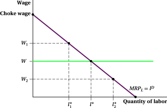
We’ve been using Samsung as an example, but this outcome is true for any firm. Its labor demand curve is its MRP_L curve because the MRP_L curve shows how much labor the firm wants to hire at any given wage.

514

515

There is another interpretation of the optimal hiring condition that can be seen if we break MRP_L into its two components, MP_L and MR:

MRP_L = MP_L × MR = W

Rearranging this condition gives

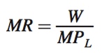
We see that at the firm’s optimal hiring level, marginal revenue equals the wage divided by the marginal product of labor. The ratio on the right-hand side reflects the cost of hiring an additional unit of labor (in dollars) divided by the number of units of output that additional labor produces. For Samsung, it’s the number of dollars (or, perhaps more accurately, Korean Won) Samsung has to spend to make each incremental smartphone, or the marginal cost of that smartphone. In other words, Samsung (and firms in general) wants to hire labor until marginal revenue equals marginal cost. This is exactly the profit-maximizing output quantity choice we discussed in Chapter 9. This equivalence implies that producing the profit-maximizing quantity also means that the firm hires the optimal amount of labor.

This connection between the output a firm makes and its optimal labor hiring implies that labor demand is a derived demand, a demand for one product (such as labor) that arises from the demand for another product (a firm’s output). This connection to the firm’s output is one conceptual way in which factor markets are distinct from markets for regular goods. When consumers are buying the typical kinds of goods we’ve been dealing with in this book, they’re seeking to maximize their utility. When firms buy factors, they’re doing so to make profits.

Like any other demand curve, the labor demand curve holds everything else constant about demand except for price (in this case, the wage). Changes in any other variable that affects labor demand show up as shifts in the labor demand curve rather than movements along it.

To understand some of those other variables, think of the separate components of the labor demand (MRP_L) curve: the marginal product of labor and marginal revenue. Forces that change either component will shift labor demand.

We saw in Chapter 6 that the MP_L depends on both the production function and the amount of capital the firm has. Changes in the production function from changes in total factor productivity (also known as technical change) will shift MP_L and, therefore, the labor demand curve. Increases in productivity increase MP_L and increase the quantity of labor demanded at each wage, thus shifting labor demand out. (Decreases in productivity have the opposite effects and shift labor demand in.)

Shifts in capital can also shift the MP_L curve, but remember for now that we are looking at labor demand in the short run when capital is fixed. We will see how changes in a firm’s capital affect the firm’s long-run demand for labor later in the chapter.

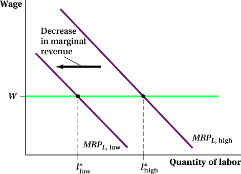
The relationship between shifts in marginal revenue and shifts in labor demand results from the fact that labor demand is a derived demand. If the demand for Samsung’s smartphones falls (as a result of changing tastes, improvements in the availability of substitutes, etc.), the price of Samsung’s smartphones will fall, and their marginal revenue will fall along with it. As shown in Figure 13.3, this decrease in marginal revenue shifts Samsung’s MRP_L curve in from MRP_L,high to MRP_L,low (where “high” and “low” denote the level of smartphone demand). Because Samsung is a wage taker, it faces a fixed market wage of W per hour. Therefore, Samsung’s quantity of labor demanded falls from l*_high to l*_low. This outcome is intuitive: If fewer people want Samsung smartphones or have lower willingness to pay for them, Samsung won’t want to hire as many workers. In general, any variable that shifts the firm’s marginal revenue curve shifts the labor demand curve.

516

We now know how labor demand is determined at the firm level. To analyze how the labor market as a whole works, we have to add up the labor demand of all firms in the economy.

In Chapter 5, we learned that a product’s market demand curve is the horizontal sum of individual consumers’ demand curves for that product. Similarly, the market demand for labor is the horizontal sum of all firms’ labor demand curves. To compute it, we pick a wage level and add up all firms’ quantity of labor demanded at that wage to get market quantity demanded at that wage. Then we repeat the process for every possible wage. The market labor demand curve must slope down because every individual firm’s labor demand curve slopes down.

The only aspect of market labor demand that can be a bit tricky has to do with the relationship between the market wage and the price of the output that firms are hiring the labor to make. When we looked at how the firm-level quantity of labor demanded changes with the market wage, we held everything else constant, including all components of the firm’s MRP_L. But for market-level labor demand, there’s a natural feedback loop between the market wage and the MRP_L of industry firms. A drop in the market wage—because it would reduce all industry firms’ costs—will also lead to a reduction in the price of the industry output. This price drop reduces the firms’ marginal revenue, shifting their MRP_L curves in. (An increase in the market wage would raise the output price and shift firms’ MRP_L curves out.) This means firms’ total response to a change in the market wage will be smaller in size than it would if there wasn’t a connection between the market wage and the output price.

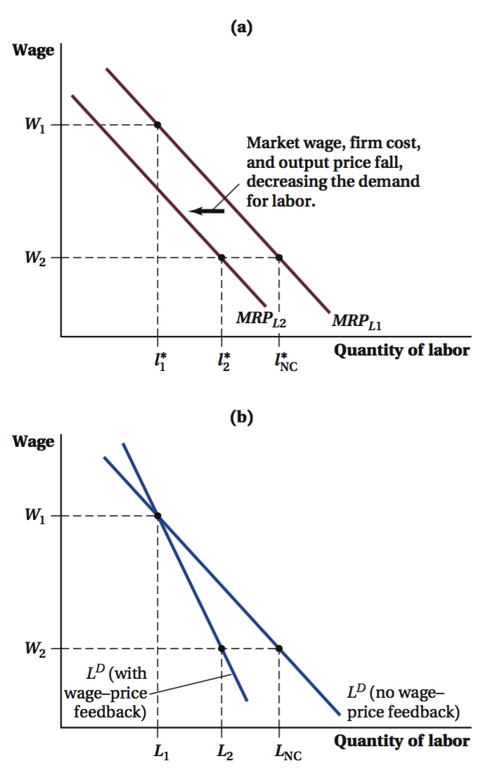
Figure 13.4 illustrates how this works. At the initial market wage and output price, an industry firm has a labor demand curve of MRP_L1. Given a market wage W₁, it hires l*₁ units of labor, as shown in panel a. If the market wage falls from W₁ to W₂, all industry firms’ costs fall and so does the output price. This reduction in marginal revenue shifts the firm’s labor demand curve to MRP_L2. Now that the market wage is W₂, the firm hires l*₂ labor units. Had there been no change in output price associated with the wage drop, the firm would have hired l*_NC (on MRP_L1) instead. At the market level, this feedback between the market wage and the output price implies that a wage drop from W₁ to W₂ increases the quantity of labor demanded from L₁ to L₂ instead of from L₁ to L_NC, as would be the case without the feedback loop. Therefore, the feedback between the market wage and output price makes the market labor demand curve steeper—less sensitive to wage changes—than it would be without the feedback, as shown in panel b.

517