Exchange efficiency shows what conditions must hold on the demand side of a market for the market to be efficient. Efficiency is also important on the production side of the economy, especially the efficiency with which inputs are allocated across the production of various goods and services. An input can be used to make one product or another, but not both simultaneously. So, which product should it be used to make? That is, how do we answer questions such as how much steel should be used to make cars instead of kitchen knives and surgical instruments, or how many workers should work in which industries? Questions like these are at the heart of the second market efficiency condition of general equilibrium, input efficiency.

Many of the tools we used to analyze exchange efficiency are also useful in analyzing input efficiency. We saw that in exchange efficiency, goods are consumed where consumers’ indifference curves are tangent to one another. Similarly, input efficiency requires an allocation of inputs across producers where their isoquants are tangent to each other. The reasoning is similar to the exchange efficiency case. At locations where producers’ isoquants are tangent to each other, no input can be transferred from one producer to another without at least one experiencing a loss in output.

Because of the similarity of the two problems, we use an Edgeworth box for our analysis. It’s just like the one we used for Elaine and Jerry, except with two producers instead of two consumers. And rather than allocating two goods between consumers, we look at how two inputs are allocated between the producers.

598

Figure 15.9 shows how 20 units of labor (horizontal axes) and 12 units of capital (vertical axes) are allocated between Cereal, Inc. (CI) and Pancake, Inc. (PI). CI’s origin, which denotes where it is using 0 units of capital and labor, is at the lower-left-hand corner of the box. Increases in CI’s use of inputs are represented by movement to the right (labor) and up (capital). CI’s isoquants—Q_C1, Q_C2, Q_C3, and so on—show the combinations of labor and capital that produce a given amount of output. PI’s origin, which denotes where it is using 0 units of capital and labor, is at the upper-right-hand corner of the box. Increases in PI’s use of inputs are represented by movements to the left (labor) and down (capital). PI’s isoquants—Q_P1, Q_P2, Q_P3, and so on—show the combinations of labor and capital that produce a given amount of output.

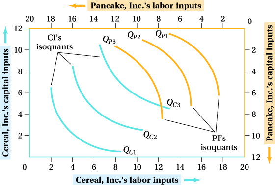
The connection between the analysis of Elaine and Jerry’s consumption bundles and the analysis of Cereal, Inc.’s and Pancake, Inc.’s input use is direct. CI’s isoquants look “normal.” PI’s isoquants also look normal if we remember that we’re looking at them from the upper-right origin. Start at an arbitrary allocation of inputs between the two firms, point F in Figure 15.10. At this point, CI is using 14 units of labor and 4 units of capital, which means that PI is using 6 units of labor and 8 units of capital. CI’s isoquant Q_C1 and PI’s isoquant Q_P1 pass through point F and enclose an area. If they use input combinations in this highlighted area, both firms can make more output than they can with input allocation F. Because both firms can make more output with the same total inputs, F cannot be a Pareto-efficient allocation of inputs.

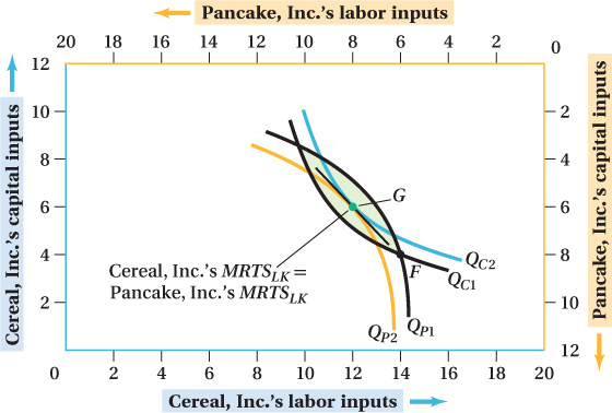
At input allocation G, where CI’s and PI’s isoquants Q_C2 and Q_P2 are tangent, there is no way to move labor and capital from one firm to the other and raise output for at least one of the firms without reducing the other firm’s output. Therefore, G is a Pareto-efficient allocation of inputs. This tangency condition also indicates that firms would experience no mutually beneficial gains from trading inputs with each other.

There are more similarities between input and exchange efficiency. Exchange efficiency implies that consumers’ marginal rates of substitution—the slopes of their indifference curves—are equal. Input efficiency implies equal slopes of producers’ isoquants. As you may recall from Chapter 6, this slope is called the marginal rate of technical substitution (MRTS), the ratio of inputs’ marginal products. For example, the MRTS between labor and capital is the ratio of the marginal product of labor to the marginal product of capital, . In our example, input efficiency requires that

599

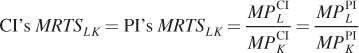
We can see this common MRTS_LK slope in Figure 15.10.

We also learned in Chapter 6 that cost-minimizing firms set their MRTS equal to the ratio of the input prices (wages and rental rates in the cases of labor and capital). Putting this all together, input efficiency implies

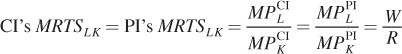
where W is the wage rate and R the capital rental rate.

Finally, a similarity exists between input and exchange efficiency in terms of the set of efficient allocations. In the exchange efficiency case, the collection of efficient goods allocations, the consumption contract curve, connects all common tangencies of the consumers’ indifference curves. The production contract curve connects all common tangencies of producers’ isoquants and contains all efficient allocations of inputs across producers (Figure 15.11).

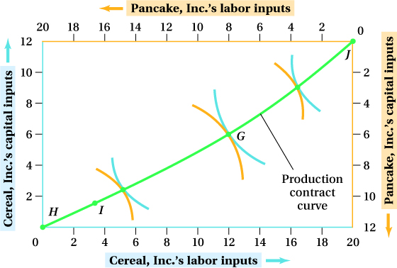
Just as different locations on the contract curve can imply very different total utility levels for Elaine and Jerry, different locations on the production contract curve correspond to disparate production quantities of cereal and pancakes. In the lower left, Cereal, Inc. uses few inputs and relatively little cereal is made, while many pancakes are produced. The opposite is true in the upper-right corner where a lot of cereal and few pancakes are produced.

600

The production contract curve generates a useful idea. Think about what various input allocations across the two firms imply about the tradeoffs between the output of either good. Imagine running along the production contract curve from the lower-left corner in Figure 15.11 to the upper-right corner, but instead of thinking about what each point corresponds to in terms of inputs, consider what each point means for cereal and pancake output.

At the very lower-left-hand corner, no inputs are used to make cereal, so cereal production is zero. Pancake output, however, is maximized at this location. This combination is plotted as point H on Figure 15.12. (For comparison, we’ve labeled the corresponding input combination in Figure 15.11.) Pancake production is positive; cereal output is zero.

601

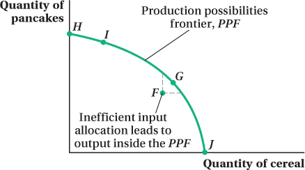
Now move up and to the right along the production contract curve to input allocation I in Figure 15.11. This move shifts inputs from pancake to cereal production. The corresponding effect on output is traced by the movement from point H to point I in Figure 15.12. Cereal output increases while pancake output falls. As we continue in the same direction along the production contract curve, cereal production rises further as pancake production drops more. When we reach the upper-right-hand corner of the Edgeworth box, cereal output is maximized, and pancake output is zero (point J).

We just traced out all the possible combinations of the cereal and pancakes that could be made if inputs are allocated efficiently across producers. The level of output for any particular good will depend on how many inputs are applied to its production, but whatever level this is, as long as the input allocation is on the production contract curve, efficiency tells us we cannot increase the output of the other good without decreasing the output of the first. The curve that connects these possible output combinations, curve HJ in Figure 15.12, is called the production possibilities frontier (PPF). Again, we see that efficiency doesn’t necessarily imply equality. Depending on the location on the production possibilities frontier, the two goods in this example can be made efficiently in very different proportions.

Inefficient input allocations will lead to cereal and pancake outputs that are inside the PPF. For example, the inefficient input allocation given by point F in Figure 15.10 might correspond to the output combination at point F in Figure 15.12. At point F, more of both goods could be made with the same total amount of inputs. The possible combinations of outputs that would be an improvement over point F (and that are attainable given the total amount of inputs available) are those contained within the wedge-shaped area in Figure 15.12. This area corresponds to the outputs that could be made by input combinations within the shaded area between Q_C1 and Q_P1 in Figure 15.10. Points on the PPF curve itself, rather than inside it, correspond to the outputs produced by efficient combinations of inputs along the production contract curve. For example, Point G in Figure 15.12 shows the output that corresponds to the efficient input allocation G in Figure 15.10.

602