15.5 Efficiency in Markets: Output Efficiency
We’ve described what must be true if exchange and input efficiency hold, and we’ve seen a lot of parallels between the two cases: common tangencies, consumer and production contract curves, and so on. While we’ve drawn analogies, however, we haven’t drawn any direct connection between the two types of efficiency.
If we think about it for a minute, though, a connection must exist. Inputs are used to make goods that are consumed. There should be a link between the efficient allocation of inputs for making different outputs and the efficient allocation of these outputs across consumers. The link is output efficiency, which involves the choice of how many units of each product the economy should make. Understanding the requirements for output efficiency requires understanding the inherent tradeoff between the production of various goods. We describe this tradeoff first, and then show how it ties together the three efficiency conditions.
The Marginal Rate of Transformation
marginal rate of transformation (MRT)
The tradeoff between the production of any goods on the market.
The production possibilities frontier, which we showed was related to the production contract curve, illustrates how much of one output must be given up to obtain one more unit of another. This tradeoff is called the marginal rate of transformation (MRT).
The MRT from pancakes to cereal, for example, is the slope of the production possibilities frontier in Figure 15.12. At point H, the frontier is relatively flat, so the MRT is small. In other words, few pancakes have to be given up to produce one more bowl of cereal. This is true because we’ve assumed (realistically) that inputs have diminishing marginal products. When all inputs are being used to make pancakes, the inputs have relatively low marginal products in pancake production, but relatively large marginal products in cereal production. At this point, shifting just a few inputs from pancake to cereal production will have a tiny impact on total pancake production but a noticeable impact on cereal production.
The opposite is true near point J. There, the inputs’ marginal products in pancake production are high and are low in cereal production. The MRT from pancakes to cereal is therefore very high. Intermediate MRT levels exist at points toward the middle of the production possibilities frontier, like G.
This logic shows how the marginal rate of transformation is related to inputs’ marginal products. We can pin down this relationship with the following thought experiment. Suppose we want to increase cereal production. To do so, we take 1 unit of labor, a worker, say, who was making pancakes at Pancake, Inc., and instead have her start working at Cereal, Inc. How much pancake output have we given up by making this shift? The marginal product of labor at Pancake, Inc.,  . How much cereal output have we gained? The marginal product of labor at Cereal, Inc.,
  . The ratio of these two values—
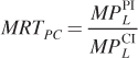
That is, the marginal rate of transformation from pancakes to cereal is the ratio of labor’s marginal product in pancake production to its marginal product in cereal production.
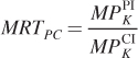
Similarly, moving a unit of capital from Pancake, Inc. to Cereal, Inc. will lead to the conclusion that the MRT is also the ratio of capital’s marginal products at the two firms:
603
We can see this equivalence another way. First, remember two things from above: The production contract curve connects all equal-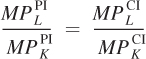 at every point on the PPF. We can rearrange this equation to show that on the PPF,
 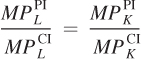 . That is, the ratios of an input’s marginal product across firms are the same for all inputs on the PPF, which is the same as saying that the MRT on the PPF is related to inputs’ marginal products.
We’ve defined the marginal rate of transformation MRT and shown that it is related to inputs’ marginal products, and through these marginal products, the MRT is related to firms’ marginal rates of technical substitution. What role do these equivalencies play in linking exchange and input efficiency?
Let’s suppose that the consumption and production sides of the market have independently come to efficient allocations. To give a specific example, say Elaine and Jerry are at an exchange-
Suppose, as well, that the economy’s production side has arrived at an efficient input allocation on the production possibilities frontier—
These outcomes result in a mismatch between consumers’ willingness to substitute one good for the other and firms’ abilities to switch from producing one to the other. To consume one more bowl of cereal, Elaine and Jerry are both willing to give up 1.5 pancakes for 1 bowl of cereal. But to produce one more bowl of cereal, society needs to only give up 1 pancake for 1 bowl of cereal. So, this economy has a disconnect between the production-
This missing link between efficiency on the consumption and production sides of the economy is output efficiency. This exists when the tradeoffs on the consumption and production sides of an economy are equal. The tradeoff on the consumption side is the marginal rate of substitution. The tradeoff on the production side is the marginal rate of transformation. Output efficiency therefore requires MRS = MRT. In our example above, if Elaine and Jerry were at an efficient allocation where their common MRS was equal to the MRT, then output efficiency would exist.
Figure 15.13 shows the production possibilities frontier from Figure 15.12 with a consumer’s indifference curves plotted with it. It doesn’t really matter whose indifference curves we plot—
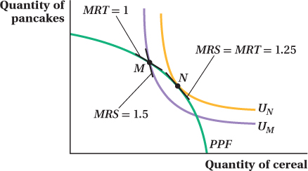
The outcome in the example above, where Elaine and Jerry’s MRS is 1.5, and the MRT is 1, is shown at point M. Exchange efficiency holds at this point because Elaine and Jerry have the same MRS. Input efficiency also holds because the output combination is on the production possibilities frontier. But, output efficiency does not hold because the indifference curve UM that goes through output combination M cuts inside the PPF. This configuration makes two important facts hold. First, output combinations above and to the right of UM are preferable to those on UM. Second, any output combination on or inside the PPF is feasible—
604
How do we reach an efficient outcome? By shifting some production from pancakes to cereal until output combination N is reached. At this combination, the indifference curve UN is tangent to the PPF. Therefore, MRS = MRT (we’ve assumed both are 1.25 in the figure), and we arrive at output efficiency. We know this is the efficient output mix because no other feasible output combination exists that would give Elaine and Jerry higher utility. Thus, output efficiency is also marked by a tangency condition.
Another way to think about the MRT = MRS condition is as a statement of that classic principle of economic optimality, that marginal benefits should equal marginal costs. As we discussed earlier, the MRS between goods equals the goods’ price ratio. Under perfect competition, as we saw in Chapter 8, a profit- . Because the marginal cost of production equals the price of an input divided by the marginal product of that input (essentially, it’s how much you have to spend on an extra amount of input to raise output by 1 unit),
 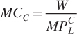 and
and 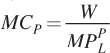 . Therefore,
 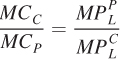 . Earlier, we showed that this ratio of the marginal products of labor is also equal to the MRT. (We would arrive at the same answer if we used the marginal products of capital because these ratios are equivalent.) Saying that output efficiency implies MRT = MRS is the same as saying that it equates the ratio of consumers’ marginal utilities of goods to the marginal costs of producing those goods.
605
figure it out 15.5
In Ecoland, producers make both televisions and clocks. At current production levels, the marginal cost of producing a clock is $50 and the marginal cost of producing a television is $150.
How many clocks must Ecoland give up if it wishes to produce another television?
What is the marginal rate of transformation from clocks to televisions in Ecoland?
At current production levels, consumers are willing to give up 2 clocks to obtain another television. Is Ecoland achieving output efficiency? Explain.
Solution:
Because the marginal cost of producing a television is 3 times that of producing a clock, Ecoland must give up 3 clocks for each television it produces.
The marginal rate of transformation (MRT) measures how much of one output must be given up to obtain one more unit of another. Therefore, the MRT from clocks to televisions is 3.
Because consumers are only willing to trade 2 clocks for a television, the marginal rate of substitution (MRS) is 2. However, output efficiency requires that MRS = MRT. Therefore, Ecoland is not achieving output efficiency.