4.4 Combining Utility, Income, and Prices: What Will the Consumer Consume?
We now have in place all the pieces necessary to figure out what a consumer will buy. We know the consumer’s preferences for bundles of goods from the utility function and its associated indifference curves. We know the consumer’s budget constraint and which bundles are feasible given her income and the goods’ prices.
Solving the Consumer’s Optimization Problem
As we mentioned in the introduction to this chapter, the choice of how much to consume (like so many economic decisions) is a constrained optimization problem. There is something you want to maximize (utility, in this case), and there is something that limits how much of the good thing you can get (the budget constraint, in this case). And as we see in the next chapter, the constrained optimization problem forms the basis of the demand curve.
Before we try to solve this constrained optimization problem, think for a minute about what makes it tricky: We must compare things (e.g., income and prices) measured in dollars and things (e.g., consumer utility) measured in imaginary units like utils that don’t directly translate into dollars. How can you know whether you’re willing to pay $3 to get an extra unit of utility? Well, you can’t, really. What you can figure out, however, is whether spending an extra dollar on, say, golf balls gives you more or less utility than spending an extra dollar on something else, like AAA batteries. It turns out that figuring out this choice using indifference curves and budget constraints makes solving the consumer’s optimization problem straightforward.
Look at the axes we use to show indifference curves and budget constraints. They are the same: The quantity of some good is on the vertical axis, and the quantity of some other good is on the horizontal axis. This arrangement is extremely important, because it means we can display indifference curves and the budget constraint for two goods in the same graph, making the consumer’s problem easier to solve.
135
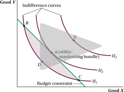
Figure 4.18 presents an example that shows a combination of indifference curves and a budget constraint. Remember, the consumer wants to get as much utility as possible from consuming the two goods, subject to the limits imposed by her budget constraint. What bundle will she choose? The bundle at point A. That’s the highest indifference curve she can reach given her budget line.
Why is A the utility-
A look at the consumer’s optimal consumption bundle A in Figure 4.18 shows that it has a special feature: The indifference curve, U2, touches the budget constraint once and only once, exactly at A. Mathematically speaking, U2 and the budget constraint are tangent at point A. As long as the original assumptions we made about utility hold, no other indifference curve we can draw will have this feature. Any other indifference curve will not be tangent, and therefore will cross the budget constraint twice or not at all. If you can draw another indifference curve that is tangent, it will cross an indifference curve shown in Figure 4.18, violating the transitivity assumption. (Give it a try—
This single tangency is not a coincidence. It is, in fact, a requirement of utility maximization. To see why, suppose an indifference curve and the budget constraint never touched. Then no point on the indifference curve is feasible, and by definition, no bundle on that indifference curve can be the way for a consumer to maximize her utility given her income.
Now suppose the indifference curve crosses the budget constraint twice. This implies there must be a bundle that offers the consumer higher utility than any on this indifference curve and that the consumer can afford. For example, the shaded region between indifference curve U1 and the budget constraint in Figure 4.18 reflects all of the bundles that are feasible and provide higher utility than bundles B, C, D, or any other point on U1. That means no bundle on U1 maximizes utility; there are other bundles that are both affordable and offer higher utility. This means that only at a point of tangency are there no other bundles that are both (1) feasible and (2) offer a higher utility level. This tangency is the utility-
136
Mathematically, the tangency of the indifference curve and budget constraint means that they have the same slope at the optimal consumption bundle. This has a very important economic interpretation that is key to understanding why the optimal bundle is where it is. In Section 4.2, we defined the negative of the slope of the indifference curve as the marginal rate of substitution, and we discussed how the MRSXY reflects the ratio of the marginal utilities of the two goods. In Section 4.3, we saw that the slope of the budget constraint equals the negative of the ratio of the prices of the two goods. Therefore, the fact that the consumer’s utility-
This economic idea behind utility maximization can be expressed mathematically. At the point of tangency,
Slope of indifference curve = Slope of budget constraint
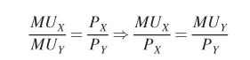
–MRSXY = –MUX/MUY = –PX/PY
MUX/MUY = PX/PY
Why are the marginal utility and price ratios equal when the consumer maximizes her utility level? If they were not equal, she could do better by shifting consumption from one good to the other. To see why, let’s say Meredith is maximizing her utility over bottles of Gatorade and protein bars. Suppose bottles of Gatorade are twice as expensive as protein bars, but she is considering a bundle in which her marginal utilities from the two goods are not 2 to 1 as the price ratio is. Say she gets the same amount of utility at the margin from another bottle of Gatorade as from another protein bar, so that the ratio of the goods’ marginal utilities is 1. Given the relative prices, she could give up 1 bottle of Gatorade and buy 2 more protein bars and doing so would let her reach a higher utility level. Why? Because those 2 extra protein bars are worth twice as much in utility terms as the lost bottle of Gatorade.
Now suppose that a bottle of Gatorade offers Meredith 4 times the utility at the margin as a protein bar. In this case, the ratio of Meredith’s marginal utilities for Gatorade and protein bars (4 to 1) is higher than the price ratio (2 to 1), so she could buy 2 fewer protein bars in exchange for 1 more bottle of Gatorade. Because the Gatorade delivers twice the utility lost from the 2 protein bars, Meredith will be better off buying fewer protein bars and more Gatorade.
It is often helpful to rewrite this optimization condition in terms of the consumer’s marginal utility per dollar spent:
Here, the utility-
10 Interestingly, the same consumer utility-
137
 See the problem worked out using calculus
figure it out 4.4

For interactive, step-
Suppose Antonio gets utility from consuming two goods, burgers and fries. His utility function is given by
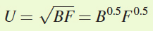
where B is the amount of burgers he eats and F the servings of fries. Antonio’s marginal utility of a burger MUB = 0.5B–0.5F0.5, and his marginal utility of an order of fries MUF = 0.5B0.5F–0.5. Antonio’s income is $20, and the prices of burgers and fries are $5 and $2, respectively. What are Antonio’s utility-
Solution:
We know that the optimal solution to the consumer’s maximization problem sets the marginal rate of substitution—
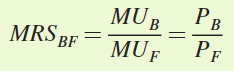
where PB and PF are the goods’ prices. Therefore, to find the utility-
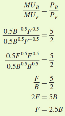
2F = 5B
F = 2.5B
This condition tells us that Antonio maximizes his utility when he consumes fries to burgers at a 5 to 2 ratio. We now know the ratio of the optimal quantities, but do not yet know exactly what quantities Antonio will choose to consume. To figure that out, we can use the budget constraint, which pins down the total amount Antonio can spend, and therefore the total quantities of each good he can consume.
Antonio’s budget constraint can be written as
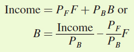
Substituting in the values from the problem gives
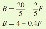
Now, we can substitute the utility-
B = 4 – 0.4F
B = 4 – 0.4(2.5B)
B = 4 – B
2B = 4
B = 2
And because F = 2.5B, then F = 5.
Therefore, given his budget constraint, Antonio maximizes his utility by consuming 2 burgers and 5 servings of fries.
Implications of Utility Maximization
The marginal-
11 Technically, this is true only of consumers who are consuming a positive amount of both goods, or who are at “interior” solutions in economists’ lingo. We’ll discuss this issue in the next section.
138
This might seem odd. First of all, we have said that you can’t compare utility levels across people. Second, even if you could—
This assertion would be true if both Jack and Meg had to consume the same bundle, but they don’t have to. They can choose how much of each good they want to consume. Because Jack likes gum a lot, he will consume so much of it that he drives down his marginal utility until, by the time he and Meg both reach their utility-
Figure 4.19 shows this outcome. To keep the picture simple, we assume Jack and Meg have the same incomes. Because they also face the same relative prices, their budget constraints are the same. Jack really likes gum relative to iTunes downloads, so his indifference curves tend to be flat: He has to be given a lot of iTunes to make up for any loss of gum. Meg has the opposite tastes. She has to be given a lot of gum to make up for giving up an iTunes download, so her indifference curves are steep. Nevertheless, both Jack and Meg’s utility-
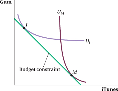
Even though Jack and Meg have the same MRSXY, the amounts of each good they consume are different. Jack, the gum lover, maximizes his utility by choosing a bundle (J) with a lot of gum and not many iTunes downloads. Meg’s optimal consumption bundle (M), on the other hand, has a lot of iTunes downloads and little gum. Again, both consumers end up with the same MRS in their utility-
139
Note that these two indifference curves cross. Although earlier we learned that indifference curves can never cross, the “no crossing” rule applies only to the indifference curves of one individual. Figure 4.19 shows indifference curves for two different people with different preferences, so the transitivity rule we talked about before doesn’t hold. If you like gum more than iTunes, and your friend likes iTunes more than, say, coffee, that doesn’t imply you have to like gum more than coffee. So the same consumption bundle (say, 3 packs of gum and 5 iTunes downloads) can offer different utility levels to different people.
A Special Case: Corner Solutions
Up to this point, we have analyzed situations in which the consumer optimally consumes some of both goods. This assumption usually makes sense if we think that utility functions have the property that the more you have of a good, the less you are willing to give up of something else to get more. Because the first little bit of a good provides the most marginal utility in this situation, a consumer will typically want at least some amount of a good.
corner solution
A utility-
interior solution
A utility-
Depending on the consumer’s preferences and relative prices, however, in some cases a consumer will not want to spend any of her money on a good. When consuming all of one good and none of the other maximizes a consumer’s utility given her budget constraint, the solution to the optimization problem is called a corner solution. (Its name comes from the fact that the optimal consumption bundle is at the “corner” of the budget line, where it meets the axis.) If the utility-
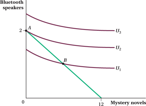
Figure 4.20 depicts a corner solution. Greg, our consumer, has an income of $240 and is choosing his consumption levels of mystery novels and Bluetooth speakers. Let’s say a hardcover mystery novel costs $20, and a Bluetooth speaker costs $120. Because speakers are more expensive than mystery novels, Greg can afford up to 12 mysteries but only 2 speakers. Nonetheless, the highest utility that Greg can obtain given his income is bundle A, where he consumes all speakers and no mystery novels.
140
How do we know A is the optimal bundle? Consider another feasible bundle, such as B. Greg can afford it, but it is on an indifference curve U1 that corresponds to a lower utility level than U2. The same logic would apply to bundles on any indifference curve between U1 and U2. Furthermore, any bundle that offers higher utility than U2 (i.e., above and to the right of U2) isn’t feasible given Greg’s income. So U2 must be the highest utility level Greg can achieve, and he can do so only by consuming bundle A, because that’s the only bundle he can afford on that indifference curve.
In a corner solution, then, the highest indifference curve touches the budget constraint exactly once, just as with the interior solutions we discussed earlier. The only difference with a corner solution is that bundle A is not a point of tangency. The indifference curve is flatter than the budget constraint at that point (and everywhere else). That means Greg’s MRS—the ratio of his marginal utility from mystery novels relative to his marginal utility from Bluetooth speakers—
figure it out 4.5
A pizza chain recently offered the following special promotion: “Buy one pizza at full price and get your next three pizzas for just $5 each!” Assume that the full price of a pizza is $10, your daily income $40, and the price of all other goods $1 per unit.
Draw budget constraints for pizza and all other goods that reflect your situations both before and during the special promotion. (Put the quantity of pizzas on the horizontal axis.) Indicate the horizontal and vertical intercepts and the slope of the budget constraint.
How is this special offer likely to alter your buying behavior?
How might your answer to (b) depend on the shape of your indifference curves?
Solution:
To draw your budget constraint, you need to find the combinations of pizza and all other goods that are available to you before and during the promotion. The starting place for drawing your budget constraint is to find its x-
and y- intercepts. Before the promotion, you could afford 4 pizzas a day ($40/$10) if you spent all of your income on pizza. This is the x-intercept (Figure A). Likewise, you could afford 40 units of all other goods per day ($40/$1) if you purchased no pizza. This is the y-intercept. The budget constraint, shown in Figure A, connects these two points and has a slope of –40/4 = –10. This slope measures the amount of other goods you must give up to have an additional pizza. Note that this is also equal to –Px/Py = –$10/$1 = –10.
Once the promotion begins, you can still afford 40 units of all other goods if you buy no pizza. The promotion has an effect only if you buy some pizza. This means the y-intercept of the budget constraint is unchanged by the promotion. Now suppose you buy 1 pizza. In that case, you must pay $10 for the pizza, leaving you $30 for purchasing all other goods. This bundle is point A on the diagram. If you were to buy a second pizza, its price would be only $5. Spending $15 on 2 pizzas would allow you to purchase $25 ($40 – $15) worth of other goods. This corresponds to bundle B. The third and fourth pizzas also cost $5 each. After 3 pizzas, you have $20 left to spend on other goods, and after 4 pizzas, you are left with $15 for other goods. These are points C and D on the diagram.
A fifth pizza will cost you $10 (the full price) because the promotion limits the $5 price to the next 3 pizzas you buy. That means if you choose to buy 5 pizzas, you will spend $35 on pizza and only $5 on other goods, as at bundle E. Now that you have again purchased a pizza at full price, you are eligible to receive the next 3 at the reduced price of $5. Unfortunately, you only have enough income for one more $5 pizza. Therefore, if you would like to spend all of your income on pizza, you can buy 6 pizzas instead of just 4.
As a result of the promotion, then, your x-intercept has moved out to 6, and your budget line has pivoted out (in a somewhat irregular way because of all the relative price changes corresponding to purchasing different numbers of pizzas) to reflect the increase in your purchasing power due to the promotion.
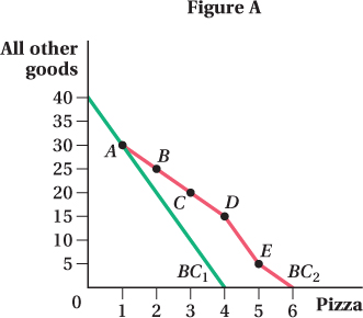
It is likely that the promotion will increase how much pizza you consume. Most of the new budget constraint lies to the right of the initial budget constraint, increasing the number of feasible bundles available to you. Because more is preferred to less, it is likely that your optimal consumption bundle will include more pizza than before.
If your indifference curves are very flat, you have a strong preference for other goods relative to pizza. For example, look at UA (Figure B). The slope of this indifference curve is relatively small (in absolute value). This means that the marginal rate of substitution of pizza for other goods is small. If your indifference curves look like this, you are not very willing to trade other goods for more pizza, and your optimal consumption bundle will likely lie on the section of the new budget constraint that coincides with the initial budget constraint. The promotion would cause no change in your consumption behavior; pizza is not a high priority for you, as indicated by your flat indifference curve.
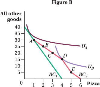
On the other hand, if your indifference curves are steeper, like UB, your marginal rate of substitution is relatively large, indicating that you are willing to forgo a large amount of other goods to consume an additional pizza. This promotion will then, more than likely, cause you to purchase additional pizzas.
141