Individual and Market Demand 5

Appendix Introduction

195

Chapter 5 Appendix

Chapter 5 Appendix: The Calculus of Income and Substitution Effects

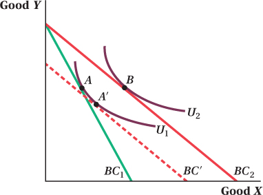
We saw in this chapter that a price change in one good influences a consumer’s consumption in two ways. The substitution effect is the change in a consumer’s optimal consumption bundle due to a change in the relative prices of the goods, holding his utility constant. The income effect is the change in a consumer’s optimal consumption bundle due to the change in his purchasing power. In the chapter, we solved for these two effects using a figure like the one below where good X is shown on the horizontal axis and good Y on the vertical axis. The consumer’s original consumption bundle is A. Consumption bundle B is the optimal bundle after a decrease in the price of X, holding the price of Y constant. Finally, bundle A′ shows what the consumer would buy if the price of X decreased but utility stayed the same as at bundle A (i.e., on indifference curve U₁). Graphically, the substitution effect is the change from bundle A to bundle A′, the income effect is the change from A′ to B, and the total effect is the sum of these two effects or the change from A to B.

The graphical approach to decomposing the income and substitution effects can be a little messy. You have to keep track of multiple budget constraints, indifference curves, and their respective shifts. The calculus links the effects we observed in the graph to the techniques we learned for solving the consumer’s problem in the Chapter 4 Appendix. Solving for these effects is a two-step process. We begin by finding the new consumption bundle B to solve for the total effect. Second, we solve for bundle A′, which will allow us to identify both the substitution and income effects.

Let’s start with a consumer with budget constraint I = P_XX + P_YY (BC₁ in the graph) and a standard Cobb–Douglas utility function U(X,Y) = X^αY^1–α, where 0 < α < 1. Point A in the figure is the solution to the constrained optimization problem:

196

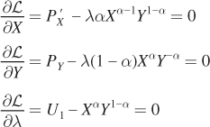
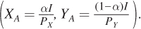
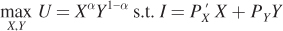
In the Chapter 4 Appendix, we derived the solution to this particular utility-maximization problem, and found that the optimal bundle A is

Now suppose that the price of good X, P_X, decreases to P_X′.The consumer has the same utility function as before, but because of the price change, his budget constraint rotates outward to 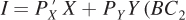on the graph). Once again, we rely on utility maximization to solve for the optimal bundle:

Because we already know the generic solution to this problem, we can plug in the new price of X to find the new optimal bundle 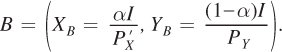This gives us the total effect of the price change on the consumer’s consumption bundle—the difference between his new consumption bundle and his original consumption bundle Note that in this instance the change in the price of X does not affect the quantity of Y the consumer purchases. That the demand for each good is independent of changes in the price of the other good is a quirk of the Cobb–Douglas utility function. This result is not necessarily true of other utility functions.

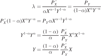
The solution to the utility-maximization problem gives us the final bundle B. But we want to know more than just the total effect of the price change on the consumption bundle. We want to decompose this total effect into its two components: the substitution and income effects. We can do this by solving for bundle A′.

What is the substitution effect? It is the effect of the change in the relative price of two goods on the quantities demanded given the consumer’s original level of utility. How can we solve for this effect? It’s easy! When we know the consumer’s original level of utility and the goods’ prices, as we do here, expenditure minimization tells us the answer to the problem. Take the consumer’s original level of utility U₁ as the constraint and set up the consumer’s expenditure-minimization problem

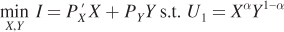
as a Lagrangian:

Write out the first-order conditions:

Solve for Y using the first two conditions:

197

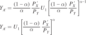
Plug this expression for Y as a function of X into the constraint to solve for bundle A′:

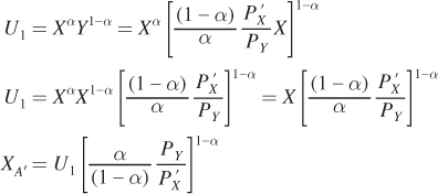
Then plug this optimal value of X into the expression for Y as a function of X from above:

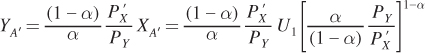
To simplify, invert the third term and combine like terms:

Solving the consumer’s expenditure-minimization problem at the new prices and original utility level gives us the third piece of the substitution/income effect puzzle: bundle A′.8 Having these three bundles (A, A′, and B) allows us to solve for the substitution and income effects. The substitution effect is the difference between the consumer’s original bundle and what he would buy at the new prices but at the old utility level, the difference between A and A′. The income effect is the difference between what he would buy at the new prices and original utility and what he buys with his new income at the new prices, the difference between A′ and B. The total effect is the sum of the substitution and income effects or the difference between A and B.

8 One way to check our answer to bundle A′ is to take the new prices, income, and utility function, and solve for the bundle using utility maximization. As we saw in the Chapter 4 Appendix, this approach will yield the same answer.

figure it out 5A.1

A sample problem will make breaking down the total effect of a price change into the substitution and income effects even clearer. Let’s return to Figure It Out 4.4, which featured Antonio, a consumer who purchases burgers and fries. Antonio has a utility function and income of $20. Initially, the prices of burgers and fries are $5 and $2, respectively.

What is Antonio’s optimal consumption bundle and utility at the original prices?
The price of burgers increases to $10 per burger, and the price of fries stays constant at $2. What does Antonio consume at the optimum at these new prices? Decompose this change into the total, substitution, and income effects.

Solution:

We solved this question in the Chapter 4 Appendix, but the answer will be crucial to solving for the total, substitution, and income effects in part (b). When a burger costs $5 and fries cost $2, Antonio’s original constrained optimization problem is

We found that Antonio consumes 2 burgers and 5 orders of fries, and his utility for this bundle is B^0.5F^0.5 = 2^0.55^0.5 = 10^0.5.
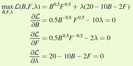
When the price of hamburgers doubles to $10 each, Antonio faces a new budget constraint: 20 = 10B + 2F. Antonio’s new utility-maximization problem is

198

Therefore, we should write his constrained optimization problem as a Lagrangian and solve for his new optimal bundle at the higher burger price:

We use the first two conditions to solve for λ and then solve for F as a function of B:

λ = 0.05B^–0.5F^0.5 = 0.25B^0.5F^–0.5

F^0.5F^0.5 = 20(0.25)B^0.5B^0.5

F = 5B

and substitute this value for F into the budget constraint:

20 = 10B + 2F

20 = 10B + 2(5B)

20 = 20B

B* = 1 burger

F* = 5B = 5(1) = 5 orders of fries

In response to the increase in the price of burgers from $5 to $10, then, Antonio decreases his consumption of burgers and leaves his consumption of fries unchanged. Therefore, the total effect of the price change is that Antonio’s consumption of burgers declines by 1 and his consumption of fries remains the same at 5.

Next, we use expenditure minimization to find the substitution and income effects. Remember that we want to find out how many burgers and fries Antonio will consume if the price of burgers is $10 but his utility is the same as his utility when burgers cost $5. His third constrained optimization problem is

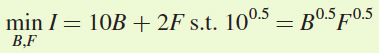
We could solve using the Lagrangian as we did above, but instead let’s use what we know about the solution to the consumer’s optimization problem and set the marginal rate of substitution of burgers for fries equal to the ratio of their prices and solve for F as a function of B:

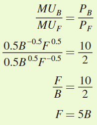
Now plug this value for F into the consumer’s utility constraint:

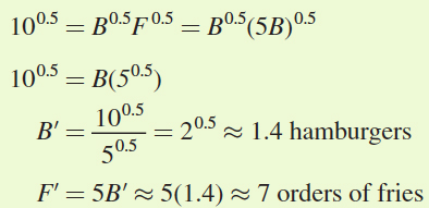
Antonio’s expenditure-minimizing bundle for the new prices and the original utility is approximately 1.4 hamburgers and 7 fries compared to his original bundle of 2 hamburgers and 5 fries. As intuition would tell you, the desired consumption of burgers decreases when burgers become relatively more expensive, while the desired consumption of fries increases as fries become relatively less expensive—that’s the substitution effect in action. In particular, Antonio’s substitution effect is to consume 0.6 fewer burgers (1.4 – 2 burgers = –0.6 burgers) and 2 more orders of fries (7 – 5 orders of fries = 2 orders of fries).

While this bundle gives Antonio the same level of utility as the original bundle, he would have to spend about $8 more to buy it [his original expenditure was $20; his new one is $10(1.4) + $2(7) = $28]. Remember, however, that Antonio doesn’t actually purchase this $28 combination of burgers and fries. It’s just a step on the way to his final consumption bundle (1 hamburger, 5 orders of fries) that we got from the utility-maximization problem above. We can use this final bundle to find the income effect. Here, the income effect is to consume 0.4 fewer burgers (1 – 1.4 burgers = –0.4 burgers) and 2 fewer orders of fries (5 – 7 orders of fries = –2 orders of fries) because the increase in the price of burgers reduces Antonio’s purchasing power. Notice that the quantity of both goods declines as his purchasing power declines. This means that, for Antonio, they are both normal goods.

In the end, the price change only changes Antonio’s consumption of hamburgers: The total effect on his consumption bundle is 1 fewer burger (1 – 2 burgers = –1 burger), which is the sum of the substitution effect (–0.6 burgers) and the income effect (–0.4 burgers). On the other hand, the total effect on his consumption of fries is zero because the substitution effect (2 more orders of fries) and the income effect (2 fewer orders of fries) exactly offset one another.

199

Let’s review what we’ve learned about decomposing the total effect of a price change into the substitution and income effects. To find the original bundle, we solve the utility-maximization problem at the original prices and income. We identify the substitution effect after a price change by solving the expenditure-minimization problem using the new prices with the original level of utility as the constraint. This tells us how a consumer’s bundle responds to a price change while leaving the consumer with the same level of utility—the substitution effect. Finally, to find the income effect, we solve the utility-maximization problem using the new prices and the consumer’s actual income. Comparing this bundle with the bundle we found using expenditure minimization tells us how consumption responds to the change in purchasing power that is caused by the price change, or the income effect.