To begin solving the firm’s cost-minimization problem, we start with the Cobb–Douglas functional form (as we did in the Chapter 4 appendix). In this case, we use the production function that relates output Q to the amount of inputs capital (K) and labor (L): Q = AK^αL^1–α, where 0 < α < 1, and where the parameter for total factor productivity, A, is greater than zero. We have been relying almost exclusively on the Cobb–Douglas functional form throughout our calculus discussions because this functional form corresponds closely with the assumptions we make about the consumer and the producer. In the context of the producer, the Cobb–Douglas production function satisfies all the assumptions we’ve made about capital, labor, and firm output, while still yielding simple formulas. In addition, we have chosen a Cobb–Douglas function with another unique property: Because the exponents on K and L (α, 1 – α) sum to 1, the production function exhibits constant returns to scale.

Before we jump into the producer’s cost-minimization problem, let’s confirm that the Cobb–Douglas production function satisfies the assumptions about the marginal products of labor and capital and the marginal rate of technical substitution (MRTS). Specifically, we need to show first that the marginal products of labor and capital are positive, and that they exhibit diminishing marginal returns. Next, we will confirm that the MRTS is the ratio of the two marginal products.

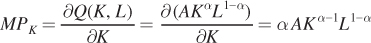
Consider first the concept of the marginal product of capital, or how much extra output is produced by using an additional unit of capital. Mathematically, the marginal product of capital is the partial derivative of the production function with respect to capital. It’s a partial derivative because we are holding the amount of labor constant. The marginal product of capital is

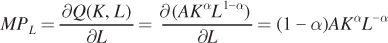
Similarly, the marginal product of labor is

240

Note that the marginal products above are positive whenever both capital and labor are greater than zero (any time output is greater than zero). In other words, the MP_L and MP_K of the Cobb–Douglas production function satisfy an important condition of production—that output increases as the firm uses more inputs.

We also need to show that the assumptions about the diminishing marginal returns of capital and labor hold true; that is, the marginal products of capital and labor decrease as the amount of that input increases, all else equal. To see this, take the second partial derivative of the production function with respect to each input. In other words, we are taking a partial derivative of each of the marginal products with respect to its input:

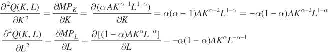
As long as K and L are both greater than zero (i.e., as long as the firm is producing output), both of these second derivatives are negative so the marginal product of each input decreases as the firm uses more of the input. Thus, the Cobb-Douglas production function meets our assumptions about diminishing marginal returns to both labor and capital.

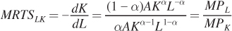
We also know from the chapter that the marginal rate of technical substitution and the marginal products of capital and labor are interrelated. In particular, the MRTS shows the change in labor necessary to keep output constant if the quantity of capital changes (or the change in capital necessary to keep output constant if the quantity of labor changes). The MRTS equals the ratio of the two marginal products. 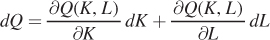To show this is true using calculus, first recognize that each isoquant represents some fixed level of output, say so that 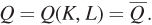Begin by totally differentiating the production function:

We know that dQ equals zero because the quantity is fixed at :

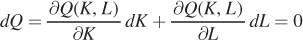
so that

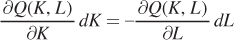
Now rearrange to get on one side of the equation:

The left-hand side of this equation is the negative of the slope of the isoquant, or the marginal rate of technical substitution.* Therefore,

1 Recall that isoquants have negative slopes; therefore, the negative of the slope of the isoquant, the MRTS, is positive.

In particular, we differentiate the Cobb–Douglas production function, Q = AK^αL^1–α, and set dQ equal to zero:

241

Again, rearrange to get on one side of the equation:

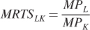
which simplifies to

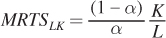
Thus, we can see that the marginal rate of technical substitution equals the ratios of the marginal products for the Cobb–Douglas production function. This also shows that the MRTS_LK decreases as the firm uses more labor and less capital, holding output constant, as we learned in the chapter. Using calculus makes it clear, however, that the rate at which labor and capital can be substituted is determined by α, the relative productivity of capital.