So far, we have only solved the firm’s cost-minimization problem for a specific quantity. In other words, we’ve assumed that the firm knows how much output it wants to produce and then decides how best to produce that quantity at the lowest cost. But it might make sense to expand our thinking about how the firm makes its production decisions. In particular, what if a firm wants to know how its optimal input mix varies with its output quantity? This is the firm’s expansion path, and it’s something we found graphically in the chapter. Recall that an expansion path shows the cost-minimizing relationship between K and L for all possible levels of output. Let’s now find the expansion path using calculus.

Consider again the firm with the familiar Cobb–Douglas production function, Q = AK^αL^1–α, and rental cost of capital and wage equal to R and W, respectively. First, write out the constrained optimization problem and the Lagrangian. Note that, unlike before, we are not going to assume that Q is a fixed level of output. In the expansion path, quantity is a variable, and that is reflected in the way we set up the constrained optimization problem below:

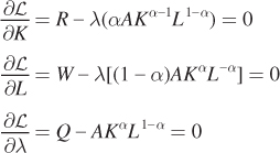
Take the first-order conditions for the Lagrangian:

As we saw earlier, solving the first two conditions gives us the optimal value of capital K* as a function of L*:

What does this tell us? Given a set of input prices, we now know the cost-minimizing amount of capital at every quantity of labor. The combination of labor and capital then determines the quantity of output. So, what have we found? The expansion path! We could also solve for the optimal amount of labor for every quantity of capital, but it’s easier to graph the expansion path with K* as a function of L*. Notice that any Cobb–Douglas production function with exponents α and (1 – α) generates a linear expansion path with slope

This linear expansion path is yet another useful property of the Cobb–Douglas functional form.

246