6.2 Production in the Short Run
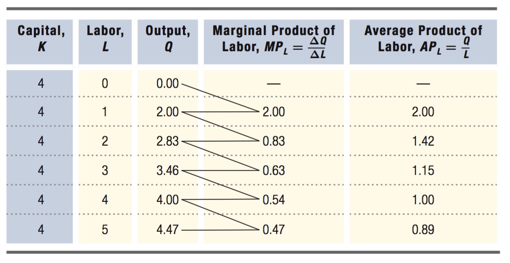
We start by analyzing production in the short run because it is the simplest case. In our earlier discussion of the assumptions of this model, we defined the short run as the period during which a firm cannot change the amount of capital. While the capital stock is fixed, the firm can choose how much labor to hire to minimize its cost of making the output quantity. Table 6.1 shows some values of labor inputs and output quantities from a short- ) at 4 units, so the numbers in Table 6.1 correspond to the production function
205
Figure 6.1 plots the short-
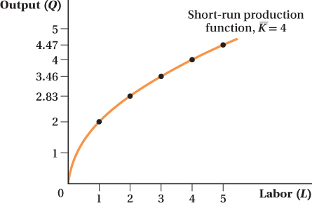
Even though capital is fixed, when the firm increases its labor inputs, its output rises. This reflects Assumption 6 above: More inputs mean more output. Notice, however, that the rate at which output rises slows as the firm hires more and more labor. This phenomenon of additional units of labor yielding less and less additional output reflects Assumption 7: The production function exhibits diminishing marginal returns to inputs. To see why there are diminishing marginal returns, we need to understand just what happens when one input increases while the other input remains fixed. This is what is meant by an input’s marginal product.
206
Marginal Product
marginal product
The additional output that a firm can produce by using an additional unit of an input (holding use of the other input constant).
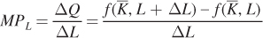
The incremental output that a firm can produce by using an additional unit of an input (holding use of the other input constant) is called the marginal product. In the short run, the marginal product that is most relevant is the marginal product of labor because we are assuming that capital is fixed at 4. The marginal product of labor (MPL) is the change in quantity (ΔQ) resulting from a 1-
MPL = ΔQ/ΔL
The marginal product of labor for our short-
diminishing marginal product
A feature of the production function; as a firm hires additional units of a given input, the marginal product of that input falls.
This diminishing marginal product of labor is the reduction in the extra output obtained from adding more and more labor; it is embodied in our Assumption 7 and is a common feature of production functions. This is why the production function curve in Figure 6.1 flattens at higher quantities of labor. A diminishing marginal product makes intuitive sense. With a fixed amount of capital, then every time you add a worker, each worker has less capital to use. If a coffee shop has one espresso machine and one worker, she has a machine at her disposal during her entire shift. If the coffee shop hires a second worker to work the same hours as the first, the two workers must share the machine and will get in each other’s way. With three workers per shift and still only one machine, the situation gets worse. A fourth worker produces a tiny bit more output, but this fourth worker’s marginal product will be smaller than the first’s. The coffee shop’s solution to this problem is to buy more espresso machines—
Keep in mind, however, that diminishing marginal returns do not have to occur all the time; they just need to occur eventually. A production function could have increasing marginal returns at low levels of labor before running into the problem of diminishing marginal product.
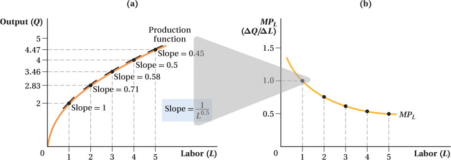
A Graphical Analysis of Marginal Product We can plot the marginal product on a graph of the production function. Recall that the marginal product is the change in output quantity that comes from adding one additional unit of input: MPL = ΔQ/ΔL. ΔQ/ΔL is the slope of the short-
207
A Mathematical Representation of Marginal Product To find MPL, we need to calculate the additional output obtained by adding an incremental unit of labor, holding capital constant. So let’s compute the firm’s increase in output when it uses L + ΔL units of labor instead of L units (holding capital constant). ΔL is the incremental unit of labor. Mathematically, MPL is
Applying this to our short-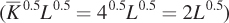 gives
gives
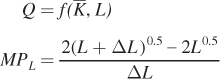
To consider what happens as we let ΔL get really tiny involves some calculus. If you don’t know calculus, however, here is the marginal product formula for our Cobb– The MPL values calculated using this formula are shown in Figure 6.2. (These values are slightly different from those in Table 6.1 because while the table sets ΔL = 1, the formula allows the incremental unit to be much smaller. The economic idea behind both calculations is the same, however.)
Average Product
average product
The quantity of output produced per unit of input.
It’s important to see that the marginal product is not the same as the average product. Average product is the total quantity of output divided by the number of units of input used to produce it. The average product of labor (APL), for example, is the quantity produced Q divided by the amount of labor L used to produce it:
APL = Q/L
208
 See the problem worked out using calculus
figure it out 6.1
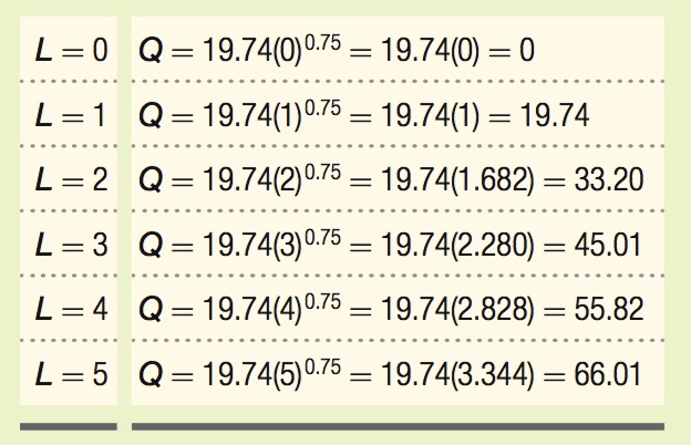
The short-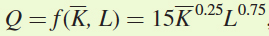 , where Q is the number of pizzas produced per hour,
  is the number of ovens (which is fixed at 3 in the short run), and L is the number of workers employed.
Write an equation for the short-
run production function for the firm showing output as a function of labor. Calculate the total output produced per hour for L = 0, 1, 2, 3, 4, and 5.
Calculate the MPL for L = 1 to L = 5. Is MPL diminishing?
Calculate the APL for L = 1 to L = 5.
Solution:
To write the production function for the short run, we plug
 into the production function to create an equation that shows output as a function of labor:
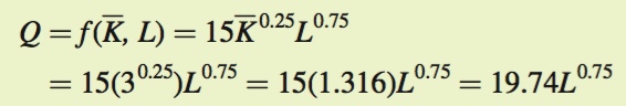
To calculate total output, we plug in the different values of L and solve for Q:
The marginal product of labor is the additional output generated by an additional unit of labor, holding capital constant. We can use our answer from (b) to calculate the marginal product of labor for each worker:
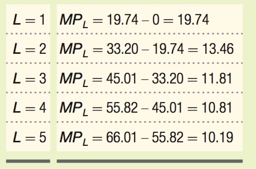
Note that, because MPL falls as L rises, there is a diminishing marginal product of labor. This implies that output rises at a decreasing rate when labor is added to the fixed level of capital.
The average product of labor is calculated by dividing total output (Q) by the quantity of labor input (L):
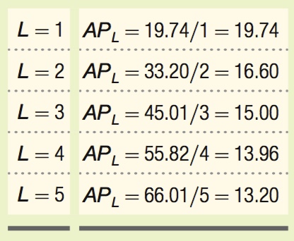
The average product of labor for our short-
209