We’ve seen how a firm minimizes its costs at the optimal production quantity. We can now use this information to illustrate how the firm’s production choices and its total costs change as the optimal production quantity changes.

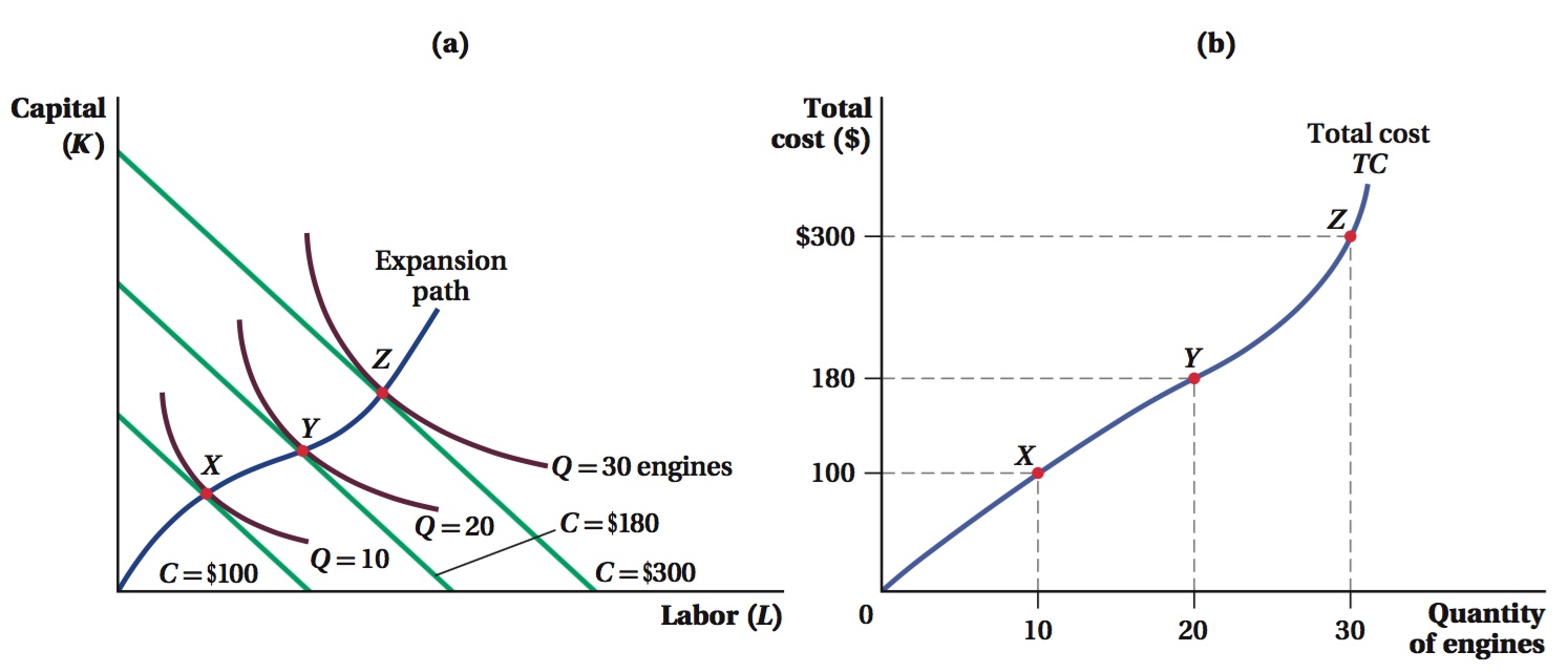
Panel a of Figure 6.15 shows sets of isoquants and isocost lines for a hypothetical firm, Ivor’s Engines. The figure illustrates three isoquants and isocost lines, but remember that there are isoquants for every possible quantity level and isocost lines for every cost level. Recall that the combination of labor and capital that minimizes the cost of producing a given quantity of output is at the tangency of an isocost line and the isoquant corresponding to that output level. The figure shows three such tangencies. On the lower left, Q = 10 is the isoquant that corresponds to input combinations that allow Ivor’s Engines to make 10 engines. This isoquant is tangent at point X to the C = $100 isocost line, so $100 is the lowest cost at which Ivor can build 10 engines. The isoquant representing input combinations that produce 20 engines, Q = 20, is tangent to the C = $180 isocost line at point Y, indicating that Ivor’s minimum cost for producing 20 engines is $180. At point Z, the Q = 30 isoquant is tangent to the C = $300 isocost line, so $300 is the minimum cost of making 30 engines.

231

The line connecting the three cost-minimizing input combinations in Figure 6.15a (as well as all the other cost-minimizing isoquant-isocost line tangencies for output levels that are not shown) is the firm’s expansion path. It illustrates how the optimal mix of labor and capital varies with total output.

The expansion path shows the optimal input combinations at each output quantity. If we plot the total cost from the isocost line and the output quantity from the isoquants located along the expansion path, we have a total cost curve that shows the cost of producing particular quantities. Panel b of Figure 6.15 gives these cost and quantity combinations for the expansion path in Figure 6.15a, including the three cost-minimizing points at 10, 20, and 30 units of output. The total cost curve is another representation of the information revealed by the expansion path. Both the total cost curve and the expansion path show how, when the firm is minimizing its costs of producing any given quantity, the firm’s minimized costs change when its output changes.

Note that the expansion path and the total cost curve that corresponds to it are for a given set of input prices (as reflected in the isocost lines) and a given production function (as reflected in the isoquants). As we saw earlier, if input prices or the production function changes, so will the cost-minimizing input combinations. Therefore, the expansion path and the total cost curve will change, too. In Chapter 7, we use the total cost curve—as derived from the expansion path—in our discussion of a firm’s cost functions.

232