7 Costs

Chapter Introduction

281

Chapter 7 Appendix

Chapter 7 Appendix: The Calculus of a Firm’s Cost Structure

We saw in this chapter that firms face a multitude of costs—from opportunity costs and sunk costs to fixed and variable costs to marginal costs and more. These costs can be obtained directly from the firm’s production function and its wage and rental rate for particular levels of output. But it is often helpful to have a more generalized form of a firm’s costs that allows us to know its cost structure at any optimal input bundle. In this appendix, we use calculus to come up with total and marginal cost curves starting from the firm’s production function.

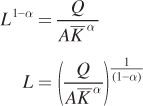
Let’s return to the firm with the Cobb–Douglas production function Q = AK^αL^1–α with wages equal to W, the rental rate of capital equal to R, and the technology parameter A. Assume 0 < α < 1, and A > 0. The firm’s total costs are

TC = RK + WL

This formula specifies the firm’s total costs when the firm produces a specific quantity and thus knows its cost-minimizing bundle of capital and labor for that particular quantity. If the firm hasn’t yet decided how much to produce, however, the firm would want to know its entire total cost curve—that is, what its total costs are at any quantity it chooses to produce. How can a firm find these costs? The firm wants to derive its total costs as a function of its demands for capital and labor. To do this, the firm first has to consider whether it is operating in the short or the long run. In the short run, capital is fixed at some level , and the firm’s production function is 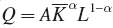. Its demand for labor in the short run is then determined by how much capital the firm has. Finding the short-run demand for labor is as simple as solving for L in the production function:

Plugging this short-run demand for labor and the fixed amount of capital ( ) into the total cost equation, the firm faces short-run total cost:

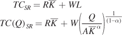
In the long run, the firm chooses the optimal amount of capital and labor, so its long-run demands for capital and labor look different. We know from the firm’s cost-minimization problem in the Chapter 6 Appendix that at a fixed quantity , the firm demands 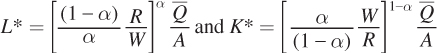. At any level of Q, then, the firm demands 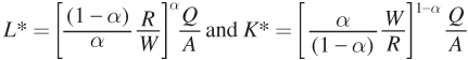, where Q is variable and not a fixed quantity.

282

These are the firm’s long-run capital and labor demand curves. As with all demand curves, these are downward-sloping: As the wage (or rental rate) increases, the firm will want to purchase less labor (or capital), all else equal. Now that we have the firm’s demands for both of its inputs, we can substitute them into the expression for total cost as a function of inputs to get the long-run total cost curve as a function of output:

TC_LR = RK + WL

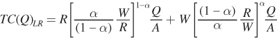
Notice that total cost increases as output and the prices of inputs increase, but that total cost decreases as total factor productivity A increases.

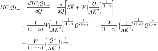
We can now also find the firm’s generalized marginal cost curve by taking the derivative of the total cost curve with respect to quantity Q. But be careful before you do this! We have to again consider whether the firm is operating in the short run or the long run. In the short run, the cost of capital is a fixed cost and will not show up in the firm’s marginal cost curve. Short-run marginal cost is only a function of the change in labor costs:

As we would expect, marginal costs increase with output in the short run. Why? Because in the short run capital is fixed. The firm can only increase output by using more and more labor. However, the diminishing marginal product of labor means that each additional unit of labor is less productive and that the firm has to use increasingly more labor to produce an additional unit of output. As a result, the marginal cost of producing this extra unit of output increases as short-run production increases, all else equal.

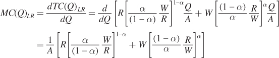
In the long run, the firm can change both inputs, and its marginal cost curve reflects the firm’s capital and labor demands. To get long-run marginal cost, take the derivative of long-run total cost with respect to Q:

Notice that this expression for marginal cost consists only of constants (A, α, W, and R). So, long-run marginal cost is constant for this production function. What is more, average total cost for this production function is exactly the same as marginal cost—you should be able to show this by dividing TC by Q. Both of these results (constant marginal cost and MC = ATC) are unique to firms with constant returns to scale. If these firms want to double output, they have to double labor and capital. This, in turn, doubles the firms’ costs, leaving average total cost—total cost divided by total inputs—unchanged. If the firm does not face constant returns to scale, these results will not hold true. In particular, a firm with decreasing returns to scale would see increasing long-run marginal costs, while a firm with increasing returns to scale faces decreasing long-run marginal costs.

283

figure it out 7A.1

Let’s revisit Figure It Out 7.4. Steve and Sons Solar Panels has a production function of Q = 4KL and faces a wage rate of $8 per hour and a rental rate of capital of $10 per hour. Assume that, in the short run, capital is fixed at .

Derive the short-run total cost curve for the firm. What is the short-run total cost of producing Q = 200 units?
Derive expressions for the firm’s short-run average total cost, average fixed cost, average variable cost, and marginal cost.
Derive the long-run total cost curve for the firm. What is the long-run total cost of producing Q = 200 units?
Derive expressions for the firm’s long-run average total cost and marginal cost.

Solution:

To get the short-run total cost function, we need to first find L as a function of Q. The short-run production function can be found by substituting into the production function: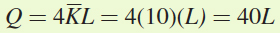

Therefore, the firm’s short-run demand for labor is

L = 0.025Q

Now plug and L into the total cost function:

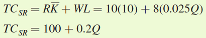
This is the equation for the short-run total cost curve with fixed cost FC equal to 100 and variable cost VC equal to 0.2Q. Notice that the fixed cost is just the total cost of capital, 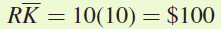. The short-run total cost of producing 200 units of output is

TC_SR = 100 + 0.2(200) = $140
Average costs are a firm’s costs divided by the quantity produced. Hence, the average total cost, average fixed cost, and average variable cost measures for this total cost function are

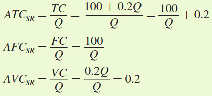
Marginal cost is the derivative of total cost with respect to quantity, or

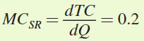
Marginal cost for Steve and Sons is constant and equal to average variable cost in the short run because the marginal product of labor is constant when capital is fixed.

284
In the long run, Steve and Sons solves its cost-minimization problem:

The first-order conditions are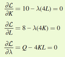

To find the optimal levels of labor and capital, we need to set the first two conditions equal to solve for K as a function of L:

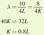
To find the firm’s long-run labor demand, we plug this expression for K as a function of L into the production function and solve for L:

Q = 4KL = 4(0.8L)L = 3.2L²

L² = 0.31Q

L = 0.56Q^0.5

To find the firm’s long-run demand for capital, we simply plug the labor demand into our expression for K as a function of L:

K = 0.8L = 0.8(0.56Q^0.5)

= 0.45Q^0.5

The firm’s long-run total cost function can be derived by plugging the firm’s long-run input demands L and K into the long-run total cost function:

TC_LR = RK + WL = 10(0.45Q^0.5) + 8(0.56Q^0.5)

= 8.98Q^0.5

Therefore, the cost for producing 200 units of output in the long run is

TC_LR = 8.98(200)^0.5 ≈ $127
We can also find the long-run marginal and average total costs for this firm: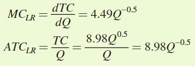

Notice that marginal cost in this case decreases as output increases. Furthermore, MC < ATC for all levels of output. This is because Steve and Sons’ production function, Q = 4KL, exhibits increasing returns to scale at all levels of output.

285