7.3 Costs and Cost Curves
We’ve seen that a firm considers its economic costs when making decisions about how much output to produce. Those economic costs include both accounting and opportunity costs so that the costs of all inputs are considered.
variable cost
The cost of inputs that vary with the quantity of the firm’s output.
total cost
The sum of a firm’s fixed and variable costs.
Economic analysis divides costs into two basic types: fixed costs and variable costs. As we learned in Chapter 6, fixed costs (FC) are costs that do not depend on how much output the firm produces. They must be paid even if the firm produces no output. Variable costs (VC) are costs that change as the firm changes its quantity of output. Every cost is either a fixed or variable cost, so a firm’s total cost (TC) is the sum of its fixed and variable costs: TC = FC + VC.
255
Fixed Cost
BMW has an assembly plant in Spartanburg, South Carolina, where the company manufactures what it calls its Sports Activity series of cross-
We often think of fixed costs as relating to capital inputs, but labor input costs can sometimes be fixed, too. For example, if BMW hires security guards to ensure that the plant is not broken into or vandalized, they work and have to be paid regardless of the factory’s output. Thus, the security guards’ wages are part of fixed cost.
If fixed costs aren’t sunk, they can be avoided, but only if the firm closes its business and exits the market completely. Exiting the market is different from producing zero output. If BMW stops production at the plant but keeps possession of the plant and its capital, it still has to pay fixed costs for its capital inputs. Even if it owns the capital, those inputs still have an opportunity cost that will be borne by the firm. To close its business completely, BMW would have to sell off its plant and all the capital within it. Only by doing that can BMW avoid paying its fixed costs.
Variable Cost
Variable cost is the cost of all the inputs that change with a firm’s level of output. When a firm needs more of an input to make more output, the payment for that input counts as a variable cost.
For every hamburger McDonald’s makes, for example, it has to buy the ingredients. Payments for buns, ketchup, and beef are included in variable cost. Most labor costs are part of variable cost as well. When more workers are needed to make more hamburgers, when more doctors are needed to treat more patients, or when more programmers are needed to write more computer code, these additional workers’ wages and salaries are added to variable cost. Some capital costs can be variable. If a construction firm has to rent more cranes to build more houses, the extra rental payments are included in variable cost. If it owns the cranes, and they wear out faster when they are used more often, this depreciation (the crane’s loss in value through use) is part of variable cost as well, because the amount of depreciation depends on the firm’s output.
Flexibility and Fixed versus Variable Costs
There is an important relationship between how easy it is for a firm to change how much of an input it uses and whether the cost of that input is considered part of fixed or variable cost. When a firm can easily adjust the levels of inputs it uses as output changes, the costs of these inputs are variable. When a firm cannot adjust how much of an input it buys as output varies, the input costs are fixed.
Time Horizon The chief factor in determining the flexibility of input levels, and therefore whether the costs of the input are considered fixed or variable, is the time span over which the cost analysis is relevant.
Over very short time periods, many costs are fixed because a firm cannot adjust these input levels over short spans of time even if the firm’s output level changes. As the time horizon lengthens, however, firms have greater abilities to change the levels of all inputs to accommodate output fluctuations. Given a long enough time span, all inputs are variable costs. There are no long-
256
Let’s return to your restaurant. On a given day, many of your costs are fixed: Regardless of how many customers come to eat, you are paying for the building, the kitchen equipment, and the dining tables. You’ve scheduled the cooks and waitstaff, so unless you can dismiss them early, you must pay them whether or not you are busy that day. About the only costs that are variable on an hour-
Over a month, more of the restaurant’s input costs become variable. You can schedule more workers on days that tend to be busy and fewer on slow days, for example. You can also choose hours of operation excluding times that are sluggish, so you only pay for full light and air conditioning when you are open and expect to be busy. All of those are variable costs now. But, you still have a one-
Over longer horizons, even the building becomes a variable cost. Next year, you can terminate the lease if business is bad. In the long run, all inputs are variable and so are the firm’s costs.
Other Factors Other features of input markets can sometimes affect how easily firms may adjust their input levels, and thus determine their relative levels of fixed and variable costs.
One such factor is the presence of active capital rental and resale markets. These markets allow firms that need certain pieces of machinery or types of buildings only occasionally (like the construction firm above that sometimes needs a crane to build houses) to pay for the input just when it’s needed to make more output. Without rental markets, firms would have to buy such inputs outright and make payments whether they use the inputs or not. By making capital inputs more flexible, rental markets shift capital costs from fixed to variable.
A great example of how rental markets have changed what costs are considered fixed and variable comes from the airline industry. In the past, airlines owned virtually all their planes. Today, however, about one-
Labor contracts can affect the fixed versus variable nature of labor costs. Some contracts require that workers be paid a specified amount regardless of how much time they spend producing output. These payments are fixed costs. For example, in the past, U.S. automakers’ contracts included “jobs banks” for laid-
257
Deriving Cost Curves
cost curve
The mathematical relationship between a firm’s production costs and its output.
When producing output, firms face varying levels of the types of costs discussed above. The nature and size of a firm’s costs are critically important in determining its profit-
There are different types of cost curves depending on what kind of costs we relate to the firm’s output. We’ll start with an example. Before we do, however, note that all cost curves are measured over a particular time period. There can be hourly, daily, or yearly cost curves, for example. The specific period depends on the context, and as we discussed, so do what cost is fixed and what cost is variable.
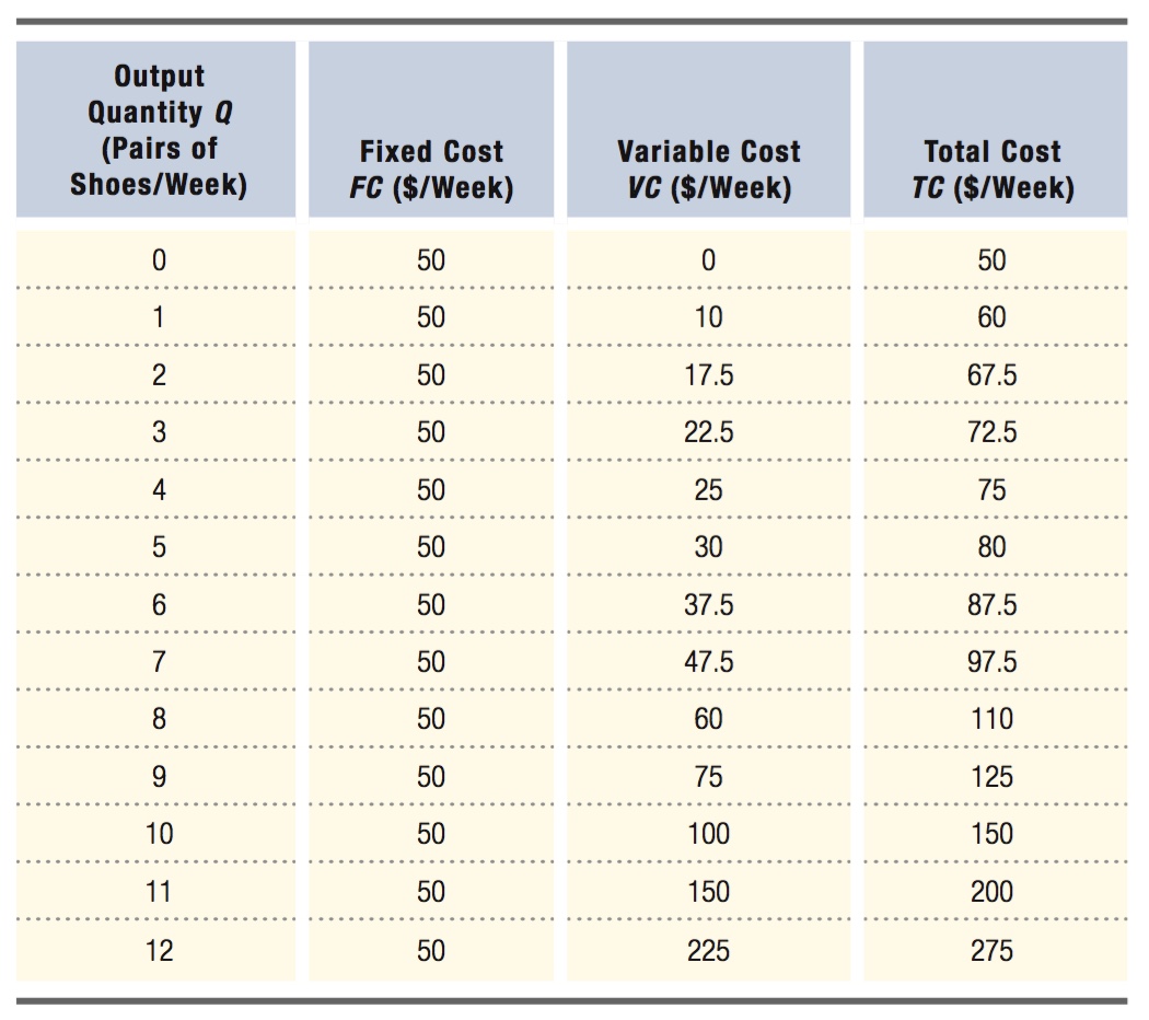
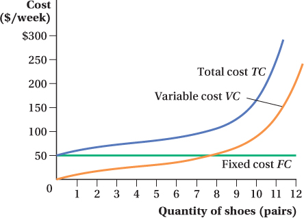
Consider the example of Fleet Foot (FF), a running shoe company. In the short run, FF uses fixed inputs (such as machinery) and variable inputs (such as labor and materials) to produce shoes. Table 7.1 shows the weekly costs for FF. These cost data are also shown graphically in Figure 7.1.
258
Fixed Cost Curve
Fixed cost does not vary with output, so it is constant and the fixed cost curve is horizontal. And because fixed cost must be paid in the short run even if the firm chooses to not produce anything, fixed cost is the same at Q = 0 as it is at every other level of output. As shown in Table 7.1, FF’s fixed cost is $50 per week, so the fixed cost curve FC in Figure 7.1 is a horizontal line at $50.
Variable Cost Curve
Variable cost changes with the output level. Fleet Foot’s variable cost rises as output increases because FF must buy more of these variable inputs. The relationship between the amount of variable inputs a firm must buy and its output means the slope of the VC curve is always positive. The shape of FF’s particular VC curve in Figure 7.1 indicates that the rate at which FF’s variable cost increases first falls and then rises with output. Specifically, the curve becomes flatter as weekly output quantities rise from 0 to 4 pairs of shoes, indicating that the additional cost of producing another pair of shoes is falling as FF makes more shoes. However, at quantities above 4 pairs per week, the VC curve’s slope becomes steeper. At these output levels, the additional cost of producing another pair of shoes is rising. We talk more about why this is the case later in the chapter.
Total Cost Curve
The total cost curve shows how a firm’s total production cost changes with its level of output. Because all costs can be classified as either fixed or variable, the sum of these two components equals total cost. In fact, as is clear in Figure 7.1, the total and variable cost curves have the same shapes and are parallel to each other, separated at every point by the amount of fixed cost. Note also that when output is zero, total cost isn’t zero; it is $50. Fleet Foot’s fixed cost must be paid in the short run even when the firm produces no output.