Problems
(Solutions to problems marked * appear at the back of this book. Problems adapted to use calculus are available online at www.macmillanhighered.com/
Consider three industries: organic onion farming, aluminum production, and car production.
Drawing on the characteristics of a competitive market outlined in the chapter, explain which of the industries named is most likely to be perfectly competitive. Be sure to explain why those industries you believe are less competitive fail to meet the criteria outlined in the chapter.
The vast majority of industries are probably not perfectly competitive. Why, then, do you suppose economics courses emphasize the study of perfect competition as much as they do?
Assume that soybean production is perfectly competitive. When we study the behavior of the firm, we assume that the demand faced by it is perfectly elastic. Yet in the marketplace, demand may be highly inelastic. Drawing on the determinants of the elasticity of demand outlined in Chapter 2, resolve this apparent paradox.
Nancy sells beeswax in a perfectly competitive market for $50 per pound. Nancy’s fixed costs are $15, and Nancy is capable of producing up to 6 pounds of beeswax each year.
Use that information to fill in the table below. (Hint: Total variable cost is simply the sum of the marginal costs up to any particular quantity of output!)
Quantity Total Revenue Fixed Cost Variable Cost Total Cost Profit Marginal Revenue Marginal Cost 0 0 15 — — 1 30 2 35 3 42 4 50 5 60 6 72 Quantity Total Revenue Fixed Cost Variable Cost Total Cost Profit Marginal Revenue Marginal Cost 0 0 15 0 15 –15 — — 1 50 15 38 53 –3 50 38 2 100 15 81 96 4 50 43 3 150 15 131 146 4 50 50 4 200 15 189 204 –4 50 58 5 250 15 257 272 –22 50 68 6 300 15 337 352 –52 50 80 If Nancy is interested in maximizing her total revenue, how many pounds of beeswax should she produce?
Nancy should produce 6 pounds of beeswax to maximize total revenue.
What quantity of beeswax should Nancy produce in order to maximize her profit?
Nancy’s maximum profit is $28; she should produce 4 pounds of beeswax to generate that profit.
At the profit-
maximizing level of output, how do marginal revenue and marginal cost compare? Marginal revenue and marginal cost are equal.
Suppose that Nancy’s fixed cost suddenly rises to $30. How should Nancy alter her production to account for this sudden increase in cost?
The marginal cost does not change, so the profit-
maximizing quantity stays the same. Suppose that the bee’s union bargains for higher wages, making the marginal cost of producing beeswax rise by $8 at every level of output. How should Nancy alter her production to account for this sudden increase in cost?
Nancy maximizes profit by producing 3 pounds of beeswax.
325
The egg industry comprises many firms producing an identical product. Supply and demand conditions are indicated in the left-
hand panel of the figure below; the long- run cost curves of a representative egg producer are shown in the right- hand panel. Currently, the market price of eggs is $2 per dozen, and at that price consumers are purchasing 800,000 dozen eggs per day. 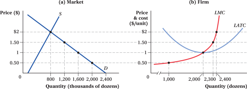
Determine how many eggs each firm in the industry will produce if it wants to maximize profit.
How many firms are currently serving the industry?
In the long run, what will the equilibrium price of eggs be? Explain your reasoning and illustrate your reasoning by altering the graphs above.
In the long run, how many eggs will the typical firm produce?
In the long run, how many firms will comprise the industry?
The diagram below depicts the revenues and costs of a firm producing vodka.
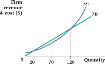
Why is total revenue represented as a straight line instead of a curve? What assumption of perfect competition does that linearity reflect?
What will the firm’s profit be if it decides to produce 20 units of output? 120 units?
Suppose the firm is producing 70 units of output and decides to cut output to 60. What will happen to the firm’s profit as a result?
Suppose the firm is producing 70 units of output and decides to increase output to 80. What will happen to the firm’s profit as a result?
At an output level of 70, draw a line tangent to the total cost curve. Does your line look similar to the total revenue curve? What does the slope of the total revenue curve indicate? What does the slope of the total cost curve indicate?
Jiang’s Pussycats sells ceramic kittens. The marginal cost of producing a particular kitten depends on how many kittens Jiang produces, and is given by the formula MC = 0.8Q. Thus, the first kitten Jiang produces has a marginal cost of $0.80, the second has a marginal cost of $1.60, and so on. Assume that the ceramic kitten industry is perfectly competitive, and Jiang can sell as many kittens as she likes at the market price of $16.
What is Jiang’s marginal revenue from selling another kitten? (Express your answer as an equation.)
Determine how many kittens Jiang should produce if she wants to maximize profit. How much profit will she make at this output level? (Assume fixed costs are zero. It may help to draw a graph of Jiang’s marginal revenue and marginal cost.)
Suppose Jiang is producing the quantity you found in (b). If she decides to produce one extra kitten, what will her profit be?
How does your answer to part (c) help explain why “bigger is not always better”?
326
Heloise and Abelard produce letters in a perfectly competitive industry. Heloise is much better at it than Abelard: On average, she can produce letters for half the cost of Abelard’s. True or False: If Heloise and Abelard are both maximizing profit, the last letter that Heloise produces will cost half as much as the last letter written by Abelard. Explain your answer.
-
Hack’s Berries faces a short-
run total cost of production given by TC = Q3 – 12Q2 + 100Q + 1,000, where Q is the number of crates of berries produced per day. Hack’s marginal cost of producing berries is 3Q2 – 24Q + 100. What is the level of Hack’s fixed cost?
Hack’s fixed cost is 1000.
What is Hack’s short-
run average variable cost of producing berries? 
If berries sell for $60 per crate, how many berries should Hack produce? How do you know? (Hint: You may want to remember the relationship between MC and AVC when AVC is at its minimum.)
AVC is minimized when it equals MC. Find this point by setting the two expressions equal and solving for Q:
3Q2 – 24Q + 100 = Q2 – 12Q + 100
2Q2 = 12Q
2Q = 12
Q = 6
The minimum value of AVC occurs when quantity is 6. To find the value of AVC at this point, substitute 6 for Q in either MC or AVC:
3(6)2 – 24(6) + 100 = (6)2 – 12(6) + 100 = 64
The minimum value of AVC is 64. Therefore, Hack should not provide any berries at a price of 60, which is below AVC. The loss-
minimizing quantity is 0. If the price of berries is $79 per crate, how many berries should Hack produce? Explain.
Begin by setting P = MC and then solve for Q:
73 = 3Q2 – 24Q + 100
3Q2 – 24Q + 27 = 0
This does not factor easily, so you will have to use the quadratic formula where a = 3, b = –24, and c = 27:
Hack would choose the larger number, because it is on the upward sloping portion of the marginal cost curve. So, he would produce 6.646 crates of berries.
Janis is one producer in the perfectly competitive pearl industry. Janis’s cost curves are shown below. Pearls sell for $100, and in maximizing profits, Janis produces 1,000 pearls per month.
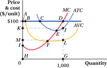
Find the area on the graph that illustrates the total revenue from selling 1,000 units at $100 each.
The rectangle ADGH represents the total revenue when selling 1,000 units at $100 each.
Find the area on the graph that indicates the variable cost of producing those 1,000 units.
The variable cost at 1,000 units is represented by the area MLGH.
Find the area on the graph that indicates the fixed cost of producing those 1,000 units.
The fixed cost of producing 1,000 units is equal to the area KJLM.
Add together the two areas you found in (b) and (c) to show the total cost of producing those 1,000 units.
The total cost of producing 1,000 units is shown by the area KJGH.
Subtract the total cost of producing those 1,000 units from the total revenue from selling those units to determine the firm’s profit. Show the profit as an area on the graph.
The profit from producing 1,000 units is represented by the area ADJK.
The diagram below depicts the cost curves for a perfectly competitive jump drive producer that is currently operating at a loss.
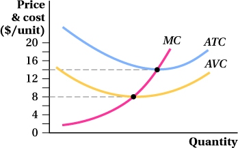
Suppose the market price of jump drives is $7. In the graph, outline an area that represents this firm’s losses if it produces where MR = MC.
If the firm in (a) instead shuts down and produces 0 units, it will lose only its fixed costs. Outline an area that represents this firm’s costs.
Which area is larger: its losses from producing where MR = MC, or its losses from producing 0 units of output? What should the firm do?
Do your answers to (a), (b), and (c) change if the price of jump drives is $11 rather than $7?
-
Marty sells flux capacitors in a perfectly competitive market. His marginal cost is given by MC = Q. Thus, the first capacitor Marty produces has a marginal cost of $1, the second has a marginal cost of $2, and so on.
Draw a diagram showing the marginal cost of each unit that Marty produces.
If flux capacitors sell for $2, determine the profit-
maximizing quantity for Marty to produce. Repeat part (b) for $3, $4, and $5.
The supply curve for a firm traces out the quantity that firm will produce and offer for sale at various prices. Assuming that the firm chooses the quantity that maximizes its profits [you solved for these in (b) and (c)], draw another diagram showing the supply curve for Marty’s flux capacitors.
Compare the two diagrams you have drawn. What can you say about the supply curve for a competitive firm?
327
Consider the following graph, which depicts the cost curves of a perfectly competitive seller of potatoes. Potatoes currently sell for $3 per pound.
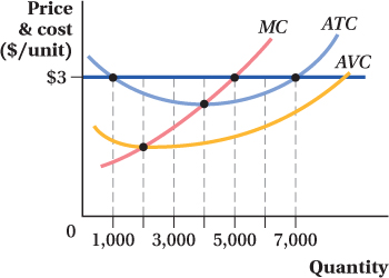
To maximize profit, how many pounds of potatoes should this seller produce?
12. The seller should produce at the level of output where MR equals MC, which occurs at 5,000 pounds of potatoes.
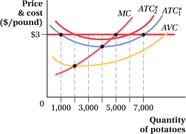
Illustrate the change in the mortgage payment by shifting the appropriate cost curves.
An increase in the mortgage payment increases the fixed cost of production, shifting the average total cost curve up.
Which curves shift? Which do not? Why?
Only the average total cost curve shifts. The average variable cost curve remains unchanged since the mortgage payment does not alter the variable cost. Similarly, the marginal cost curve is not affected by the increase in the fixed cost.
How does the change in interest rates affect the grower’s decision on how many potatoes to produce?
The change in interest rates has no effect on the producer’s decision of how many potatoes to produce in the short run because MC does not shift. (However, if the increased interest rate will increase the total cost of production above total revenue, leading to a negative economic profit, then the potato grower would shut down in the long run.)
What happens to the potato grower’s profit as a result of the increased interest rate?
The potato grower’s profit decreases. The total revenue remains unchanged but the total cost of production increases as a result of the increase in fixed cost.
How does the change in interest rates affect the shape and/or position of the grower’s short-
run supply curve? The grower’s short run supply is the MC curve above AVC. Since neither the MC curve nor the AVC curve shifted, the short run supply curve is unaffected.
Suppose that the potato grower’s bank ratchets up the interest rate applicable to the grower’s adjustable-
rate mortgage loan. This increases the size of the potato grower’s monthly mortgage payment. Five hundred small almond growers operate areas with plentiful rainfall. The marginal cost of producing almonds in these locations is given by MC = 0.02Q, where Q is the number of crates produced in a growing season. Three hundred almond growers operate in drier areas where costly irrigation is required. The marginal cost of growing almonds in these locations is given by MC = 0.04Q.
Find the individual supply curve for each type of almond grower. (Hint: Remember that the supply relationship expresses the quantity brought to market at various prices. Remember also that for a perfectly competitive firm, P = MR.)
“Add up” the individual supply curves to derive the market supply curve.
If the market demand for almonds is Qd = 105,000 – 2,500P, what will the equilibrium price of almonds be? The equilibrium quantity?
How many almonds will each type of almond grower produce at that price?
Verify that the total production of all almond growers equals the equilibrium quantity you found in part (c).
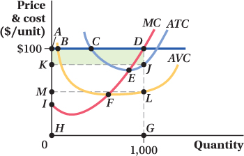
Consider Janis the pearl producer with cost curves as shown below. Janis produces 1,000 pearls when the price of pearls is $100.

What is the area of producer surplus earned by Janis if the price of pearls is $100?
Explain why areas ADI and ADLM must be equal.
For the past nine months, Iliana has been producing artisanal ice creams from her small shop in Chicago. She’s just been breaking even (earning zero economic profit) that entire time. This morning, the state Board of Health informed her that it is doubling the annual fee for the dairy license under which she (and other ice cream makers) operates, retroactive to the beginning of her operations.
In the short run, how will this fee increase affect Iliana’s output level? Her profit?
In the long run, how will this fee increase affect Iliana’s output level?
Suppose that instead of doubling the annual fee for a license, the state Board of Health required Iliana (and other ice cream makers) to treat every pint of ice cream to prevent the growth of bacteria. How would this regulation affect Iliana’s production decision and profit in both the short and long run?
Martha is one producer in the perfectly competitive jelly industry. Last year, Martha and all of her competitors found themselves earning economic profits.
If entry and exit from the jelly industry are free, what do you expect to happen to the number of suppliers in the industry in the long run?
Because of the entry/exit you described in part (a), what do you expect to happen to the industry supply of jelly? Explain.
As a result of the supply change you described in part (b), what do you expect to happen to the price of jelly? Why?
As a result of the price change you indicated in part (c), how will Martha adjust her output?
328
-
The canola oil industry is perfectly competitive. Every producer has the following long-
run total cost function: LTC = 2Q3 – 15Q2 + 40Q, where Q is measured in tons of canola oil. The corresponding marginal cost function is given by LMC = 6Q2 – 30Q + 40. Calculate and graph the long-
run average total cost of producing canola oil that each firm faces for values of Q from 1 to 10. The long-
run average total cost of producing canola oil is 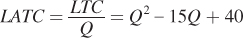
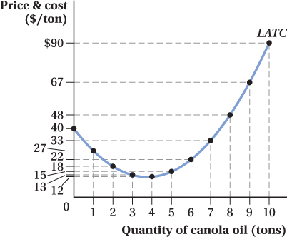
What will the long-
run equilibrium price of canola oil be? The long-
run equilibrium price of canola oil is approximately $12, which is the minimum of the LATC curve. How many units of canola oil will each firm produce in the long run?
Each firm will produce the quantity of canola oil that corresponds to the minimum point on the LATC curve, that is, 4 tons of canola oil.
Suppose that the market demand for canola oil is given by Q = 999 – 0.25P. At the long-
run equilibrium price, how many tons of canola oil will consumers demand? Using the demand function, we get
QD = 999 – 0.25P = 999 – 0.25 × 12 = 996
SB-
14 At the long-
run equilibrium price, consumers will demand approximately 996 tons of canola oil. Given your answer to (d), how many firms will exist when the industry is in long-
run equilibrium? Since each representative firm supplies 4 tons of canola oil, the number of suppliers in the long-
run equilibrium will be 
Suppose that the restaurant industry is perfectly competitive. All producers have identical cost curves, and the industry is currently in long-
run equilibrium, with each producer producing at its minimum long- run average total cost of $8. If there is a sudden increase in demand for restaurant meals, what will happen to the price of restaurant meals? How will individual firms respond to the change in price? Will there be entry into or exit from the industry? Explain.
In the market as a whole, will the change in the equilibrium quantity be greater in the short run or the long run? Explain.
Will the change in output on the part of individual firms be greater in the short run or the long run? Explain and reconcile your answer with your answer to part (b).
Suppose that the market for eggs is initially in long-
run equilibrium. One day, enterprising and profit- hungry egg farmer Atkins has the inspiration to fit his laying hens with rose- colored contact lenses. His inspiration is true genius— overnight his egg production rises and his costs fall. Will Farmer Atkins be able to leverage his inspiration into greater profit in the short run? Why?
Farmer Atkin’s right-
hand man, Abner, accidentally leaks news of the boss’ inspiration at the local bar and grill. The next thing Farmer Atkins knows, he’s being interviewed for the NBC evening news. What short- run adjustments do you expect competing egg farmers to make as a result of this broadcast? What will happen to the profits of egg farms? In the long run, what will happen to the price of eggs? What will happen to the profits of egg producers (including those of Farmer Atkins)?
In the long run, who reaps the greatest benefit from Atkins’s technological breakthrough: egg producers or egg consumers? Explain the role that competition plays in the distribution of those benefits in the transition between the short and long run.
General supply and demand analysis suggests that, in the short run, a decrease in demand causes the price of a good to fall.
Is the same assertion true (that decreases in demand cause prices to fall) in the long run?
Is it possible that a decrease in demand could actually cause prices to increase in the long run? If so, explain your reasoning.
Suppose that eggs are produced competitively and the egg industry is a constant cost industry.
Fill in the table with appropriate responses (increases, decreases, no change) in response to each of the following events:
Which event has a permanent effect on the price of eggs, and which does not?
How would your answer to (b) change if the egg industry were a decreasing cost industry?
Event Short- Run Effect on Price Long- run Effect on Price Demand for eggs increases Cost of corn (an input into egg production) decreases -
Assume that the ice cream industry is perfectly competitive. Each firm producing ice cream must hire an operations manager. There are only 50 operations managers that display extraordinary talent for producing ice cream; there is a potentially unlimited supply of operations managers with average talent. Operations managers are all paid $200,000 per year.
The long-
run total cost (in thousands of dollars) faced by firms that hire operations managers with exceptional talent is given by LTCE = 200 + Q2, where Q is measured in thousands of 5- gallon tubs of ice cream. The corresponding marginal cost function is given by LMCE = 2Q, and the corresponding long- run average total cost is LATCE = 200/Q + Q. The long-
run total cost faced by firms that hire operations managers with average talent is given by LTCA = 200 + 2Q2. The associated marginal cost function is given by LMCA = 4Q, and the corresponding long- run average total cost is LATCA = 200/Q + 2Q.
329
Derive the firm supply curve for ice cream producers with extraordinary operations managers.
Derive the firm supply curve for ice cream producers with average operations managers.
The minimum LATCA (for firms with average operations managers) is $40, achieved when those firms produce 10 units of output. The minimum LATCE (for firms with exceptional operations managers) is $28.28, achieved when those firms produce 14 units of output. Explain why, given only that information, it is not possible to determine the long-
run equilibrium price of 5- gallon tubs of ice cream. Referring to part (c), suppose that you know that the market demand for ice cream is given by Qd = 8,000 – 100P. Explain why, in the long run, that demand will not be filled solely by firms with extraordinary managers. (Hint: Derive the industry supply of extraordinary producers and then use the demand curve to determine the equilibrium price. Can that price persist in the long run?)
In part (d), you explained why the supply side of the market will consist of both firms with extraordinary managers and firms with average managers. What will the long-
run equilibrium price of ice cream be? At the price you determined in part (e), all 50 firms with extraordinary managers will find remaining in the industry worthwhile. How many firms with average managers will also remain in the industry?
At the price you determined in part (e), how much profit will a firm with an average manager earn?
At the price you determined in part (e), how much profit will a firm with an extraordinary manager earn? How much economic rent will that talented manager generate for her firm?
 Work this problem with calculus