8 Supply in a Competitive Market

8.2 Profit Maximization in a Perfectly Competitive Market

profit

The difference between a firm’s revenue and its total cost.

We just saw that Ty—and, by extension, any perfectly competitive firm—sells at the price set by the market. Although perfectly competitive firms are price takers, they do have one decision to make: the quantity to supply. Economists usually assume firms choose their actions—such as how much output to produce—to maximize profits. Profit is the difference between a firm’s revenue and its total cost. What does it mean to maximize profit? A firm does this by choosing the output level at which the difference between its total revenue and its total cost is largest. In this section, we will see that a perfectly competitive firm maximizes its profit when it produces the quantity of output at which the marginal cost of production equals the market price.

291

Total Revenue, Total Cost, and Profit Maximization

There are two basic elements to profit: revenue and cost. In general, these are both affected by a firm’s decisions about how much output to produce and the price it will charge for its output. Because perfectly competitive firms take the market price as given, we only need to focus on the choice of output.

Mathematically, let’s denote the profit a firm makes as π. The profit function is total revenue TR minus total cost TC (each of which is determined by the firm’s output quantity):

π = TR – TC

To figure out the level of output that maximizes profit, think about what happens to total cost and total revenue if the firm decides to produce one additional unit of output. Or, put differently, determine the firm’s marginal cost and marginal revenue.

We know from Chapter 7 that marginal cost is the addition to total cost of producing one more unit of output:

MC = ΔTC/ΔQ

Marginal cost is always greater than zero—it takes more inputs to make more output.

marginal revenue

The additional revenue from selling one additional unit of output.

Revenues equal the good’s price times the quantity produced. A firm’s marginal revenue is the additional revenue it gets from selling one additional unit of output:

MR = ΔTR/ΔQ

A perfectly competitive firm’s marginal revenue is the market price for the good. To see why, remember that these firms can only sell their goods at the market price P. Therefore, the extra revenue they obtain from selling each additional unit of output is P. This is really important, and so we’ll repeat it here: In a perfectly competitive market, marginal revenue equals the market price; that is, MR = P:

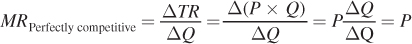
Think about what this outcome implies. Total revenue is P × Q. When a firm is a price taker, P does not change no matter what happens to Q. For a price taker, P is a constant, not a function of Q.

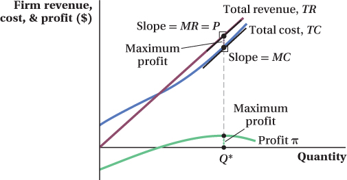
This fact means that a perfectly competitive firm’s total revenue is proportional to its output. If output increases by 1 unit, total revenue increases by the price of the product. For this reason, a perfectly competitive firm’s total revenue curve is a straight line from the origin, as shown in Figure 8.2. For example, if Ty sells another dozen eggs, his total revenue rises by the market price of $2.25. And if he keeps selling more, each additional dozen increases total revenue by another $2.25.

Figure 8.2: Figure 8.2 Profit Maximization for a Perfectly Competitive Firm

Figure 8.2: Because a perfectly competitive firm faces a constant market price, its total revenue curve is a straight line from the origin with a slope equal to the marginal revenue, or the price. At the quantity Q*, the slope of the total revenue curve (price) equals the slope of the total cost curve (marginal cost), and the firm is maximizing profit.

As we’ll see in Chapter 9, in market structures other than perfect competition, the price decreases as the quantity the firm produces increases. This introduces an additional factor into our marginal revenue calculation for firms in those other types of markets. The price reduction doesn’t happen in perfectly competitive markets because a firm does not affect the market price with its output choice. So remember, this case of marginal revenue equaling the market price is special: It only applies to firms in perfectly competitive markets.

292

How a Perfectly Competitive Firm Maximizes Profit

Now that we know the marginal cost and marginal revenue, how does our firm maximize profit in a perfectly competitive market? We know that total cost is always going to rise when output increases (as shown in Figure 8.2)—that is, marginal cost is always positive. Similarly, we know that the firm’s marginal revenue here is constant at all quantities and equal to the good’s market price. The key impact of changing output on the firm’s profit depends on which of these marginal values is larger. If the market price (marginal revenue) is greater than the marginal cost of making another unit of output, then the firm can increase its profit by making and selling another unit, because revenues will go up more than costs. If the market price is less than the marginal cost, the firm should not make the extra unit. The firm will reduce its profit by doing so because while its revenues will rise, they won’t rise as much as its costs. The quantity at which the marginal revenue (price) from selling one more unit of output just equals the marginal cost of making another unit of output is the point at which a firm maximizes its profit. This point occurs at Q* in Figure 8.2. There, the slope of the total revenue curve (the marginal revenue—here, the market price) equals the slope of the total cost curve (the marginal cost at Q*). In mathematical terms, the profit-maximizing level of output occurs where marginal revenue (here, price) equals marginal cost:

MR = P = MC

∂ The appendix at the end of Chapter 9 uses calculus to solve the perfectly competitive firm’s profit-maximization problem.

A firm should increase production as long as revenue increases by more than cost (i.e., when MR = P > MC). Conversely, a firm should decrease production if cost increases by more than revenue (i.e., when MR = P < MC).1

293

It should be clear from this discussion why cost plays such an important role in determining a firm’s output (and this is true for a firm in any type of market structure): It is half of the firm’s profit-maximization story. As cost changes, so does the firm’s profit-maximizing output. In the next several chapters (which examine firms that are not perfectly competitive), we will learn how the firm’s profit maximization is affected by the relationship between price and marginal revenue.

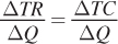
The analysis we’ve just completed shows that the output decision is fairly easy for the firm in a perfectly competitive market: It increases output until marginal cost equals the market price. If marginal cost rises with output—and we talked in Chapter 7 about the reasons why we might expect this—there will be a certain output level at which marginal cost rises to the market price. This is the profit-maximizing output level of a firm in perfect competition.

The P = MC result is extremely useful because, by linking the market price to the firm’s cost curve (or, more precisely, its marginal cost curve), we can determine how a competitive firm’s output changes when the market price changes. Consider a firm with the marginal cost curve shown in Figure 8.3. If the market price is initially P₁, then the firm’s demand and marginal revenue curve is horizontal at that price. The firm will maximize profit by setting MR = P₁ = MC and producing an output of Q*₁. If the market price increases to P₂, the firm should increase its production to output Q*₂. Why? Because the firm now faces a horizontal demand and marginal revenue curve at P₂, it should produce up to the point where marginal cost equals the market price. If price rises to P₂ and the firm continues to produce only Q₁, it could be selling those units between Q₁ and Q*₂ at a marginal revenue level (the new market price P₂) that is higher than its marginal costs. These extra sales would raise the firm’s profit.

Figure 8.3: Figure 8.3 Profit Maximization for a Perfectly Competitive Firm Occurs Where MR = P = MC

Figure 8.3: At the initial market price P₁, the perfectly competitive firm is maximizing profit at Q*₁, where P = MC. If price increases to P₂, the firm should increase output to Q*₂. If, instead, price decreases to P₃, the firm is maximizing profit at Q*₃.

If the market price instead decreases from P₁ to P₃, the firm should reduce its quantity to Q*₃, which has a lower marginal cost equal to P₃. If the firm does not make this change, it will be producing those units between Q*₃ and Q₁ at a loss because marginal revenue for those units would be lower than marginal cost.

Application: Do Firms Always Maximize Profits?

You’ve probably heard stories of CEOs who spend firm money on lavish offices, parties, or other perks. While these CEOs enjoy their spending sprees, it seems far-fetched to think that their behavior benefits the companies’ shareholders by increasing profits.

294

Given such stories, can we really assume that firms maximize profits? It is easiest to see why a small firm would want to maximize profits: Because the manager is usually the owner of the firm, maximizing the firm’s profits directly affects her personally. But larger firms are typically run by people other than the owners. As a result, their managers may be tempted to engage in behavior that does not maximize profits. These profit-killing actions don’t have to be as blatant as the kind of stories that make the news. A manager might want to raise short-run profit if her compensation package is based on it, at the expense of reductions in future profit. These missed profits could be recognized only after the manager has left the company—or never missed at all, because it can be difficult to tell what profits should be. Or, managers might undertake mergers and acquisitions that grow management’s power but that cost the acquiring firm (and its shareholders) more than the acquisition is worth.

Although managers may sometimes take actions that aren’t profit-maximizing, there are mechanisms in place to minimize the impact of such actions. These include activist shareholders, a nosy financial press, and even the occasional academic economist, who takes it upon herself to look over the shoulders of firms’ managers and scrutinize their behavior.

2Steven N. Kaplan and Bernadette A. Minton, “How Has CEO Turnover Changed?” International Review of Finance 12, no. 1 (2012): 57–87.

Profit maximization can probably be driven most directly by strong boards of directors who will confront management on behalf of the shareholders or other companies who are willing to buy up mismanaged firms and replace their executives. Economists Steven Kaplan and Bernadette Minton found evidence of these forces at work among large U.S. companies. The average CEO at these firms had been on the job less than seven years, and Kaplan and Minton found that the likelihood that a CEO stayed on the job was related to how well the company was performing relative to its industry competitors and to companies in other industries. Interestingly, these relationships held whether the CEO’s departure was publicly labeled at the time as forced or unforced—suggesting that quite a bit of “voluntary” CEO resignations are anything but.2

These forces tend to push wayward managers back toward maximizing profits, as shareholders (the owners of the capital) would desire. Even if these mechanisms fail, the competitive market itself pushes firms to maximize profit. Firms that maximize profits (or get as close to that as possible) will succeed where firms with profit-killing managers do not. Firms that maximize profits will attract additional capital more easily, have more money to invest, and take away market share from firms that fail to maximize profits. Firms that consistently fail to maximize profits will eventually be driven out of business by more profitable competitors.

Measuring a Firm’s Profit

A profit-maximizing firm in a perfectly competitive industry maximizes its profit by producing the quantity at which P = MC. But this doesn’t tell us anything about the level of profit the firm is earning (or even if it is positive) at this point. To measure profit π, we subtract total cost (TC) from total revenue (TR):

π = TR – TC

Panel a of Figure 8.4 shows the firm’s average total cost curve, its marginal cost curve, and its demand (marginal revenue) curve. The firm’s total revenue equals the area of the rectangle with height P and base Q*. Its total cost is the area of the rectangle with height ATC* (ATC at the profit-maximizing level of output Q*) and base Q*. Because total revenue is greater than total cost at Q*, the firm is earning a positive level of profit. Substituting the equations for TR and TC into the equation for profit, we see that

295

π = TR – TC

= (P × Q) – (ATC × Q)

= (P – ATC) × Q

Therefore, the firm’s profit can be seen in Figure 8.4 as the rectangle with height (P – ATC*) and base equal to the profit-maximizing quantity Q*.

The profit equation tells us that profit π = (P – ATC) × Q, and profit is positive only when P > ATC*. If P = ATC*, profit is zero, and when P < ATC*, profit is negative. These scenarios are shown in panels b and c of Figure 8.4 . Panel b shows that a firm earns zero profit when P = ATC* = MC. In Chapter 7, we learned that MC = ATC only when ATC is at its minimum. (Remember this fact! It will become very important to us toward the end of this chapter.) Panel c of Figure 8.4 shows a firm earning negative profit because P < ATC*. The obvious question is, why would a firm produce anything at a loss? We answer that question in the next section.

Figure 8.4: Figure 8.4 Measuring Profit

Figure 8.4: Given a firm’s marginal cost curve MC, average total cost curve ATC, and market price P, the firm’s profit can be measured by the area of the rectangle with length Q* and height (P – ATC*).

Figure 8.4: (a) A firm facing a market price above its average total cost curve at Q* will earn a positive economic profit, π > 0.
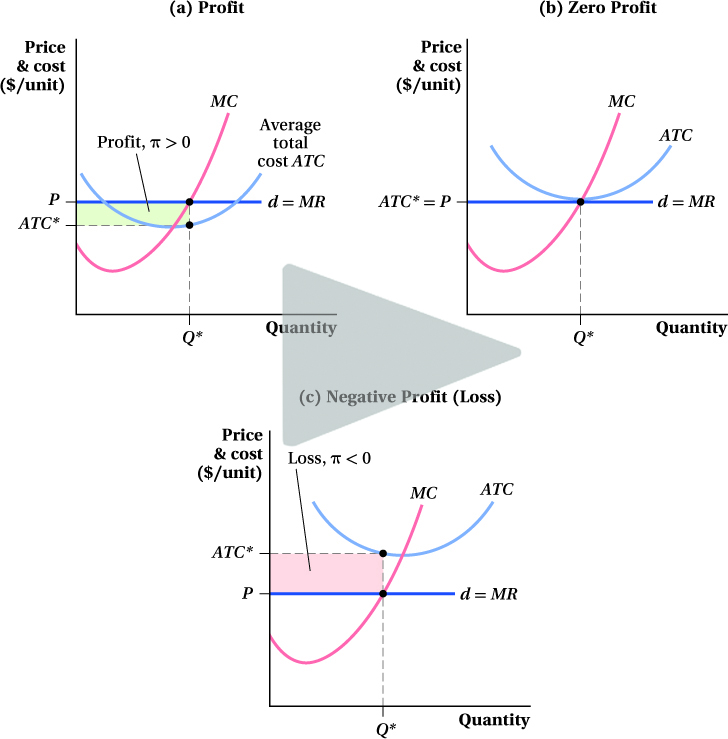
(b) A firm facing a market price equal to its average total cost at Q* earns zero economic profit.
(c) A firm with average total cost above the market price, at Q*, will earn negative economic profit (loss), π < 0.

296

See the problem worked out using calculus

figure it out 8.1

Suppose that consumers see haircuts as an undifferentiated good and that there are hundreds of barbershops in the market. The current market equilibrium price of a haircut is $15. Bob’s Barbershop has a daily short-run total cost given by TC = 0.5Q². The associated marginal cost curve is MC = Q.

How many haircuts should Bob give each day if he wants to maximize profit?
If the firm maximizes profit, how much profit will it earn each day?

Solution:

Firms in perfect competition maximize profit by producing the quantity for which P = MC:

P = MC

15 = Q
If Bob gives 15 haircuts and charges $15 for each, the total revenue will be

TR = P × Q

= $15 × 15 = $225

We can use the firm’s total cost function to find the total cost of producing 15 haircuts:

TC = 0.5Q² = 0.5(15)² = $112.50

Since profit is TR – TC,

π = $225 – $112.50 = $112.50 per day

If Profit Is Negative, Should a Firm Shut Down? How does a perfectly competitive firm know if it is better off operating at a loss or shutting down and producing zero output? (Remember that shutting down in the short run is not the same thing as exiting the industry, because firms have some fixed costs they still must pay if they shut down in the short run.) The answer (continue to operate at a loss or shut down) depends on the firm’s costs and revenues under each scenario. Table 8.2 shows the information the firm needs to make its decision.

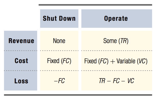
Table 8.2 Deciding Whether to Operate at a Loss or Shut Down in the Short Run

If the firm decides to shut down in the short run and produce nothing, it will have no revenue. But, because it still must pay its fixed cost, its loss will exactly equal that fixed cost:

π_{shut down} = TR – TC = TR – (FC + VC)

= 0 – (FC + 0) = –FC

If the firm continues to operate at a loss in the short run, it will accumulate some revenue, but will have to pay both fixed and variable costs. The profit from operating is the difference between total revenue and fixed and variable costs:

π_operate = TR – TC = TR – FC – VC

Comparing the two profits shows which is better:

π_operate – π_{shut down} = TR – FC – VC – (–FC)

= TR – VC

Therefore, in the short-run, a firm should operate as long as its revenue is greater than or equal to its variable cost, not its total cost (TR ≥ VC). That’s because fixed cost needs to be paid whether the plant operates or not, so it doesn’t enter into the operate/shut-down decision. Making enough revenue to cover the firm’s variable cost is sufficient to justify operating in the short run, even if the firm can’t cover all of its fixed cost, because it would lose more money if it shut down. However, if the firm has total revenue that is lower than its variable cost (TR < VC), the firm should shut down. It can’t cover its variable cost at this point and loses money on every unit it sells. Like the old joke, if you lose money on every unit, you can’t make it up on volume.

297

The operate-or-shut-down decision can be summed up as follows:

Operate if TR ≥ VC.

Shut down if TR < VC.

Figure 8.5 illustrates these rules. It shows a perfectly competitive firm’s average total cost, average variable cost, marginal cost, and marginal revenue (market price) curves. In the case shown in the figure, the firm is losing money because TR < TC, but it continues to operate because TR > VC. How can we tell this from the figure? We know that TR is the area of a rectangle where P is the height and Q* is the base (TR = P × Q), and VC is the rectangle with height AVC* (AVC at Q*) and base Q* (VC = AVC × Q). Both TR and AVC contain Q*, so this quantity cancels out and plays no role in the operate/shut-down decision. We can now rewrite the rules above in terms of the market price P facing the firm and its average variable cost AVC* at the profit-maximizing (or in this case loss-minimizing) quantity:

Operate if P ≥ AVC*.

Shut down if P < AVC*.

Therefore, the firm should keep operating as long as the market price is at least as large as its average variable cost at the quantity where price equals its marginal cost. Keep in mind that these rules apply to all firms in all industries in any type of market structure.

Figure 8.5: Figure 8.5 Deciding Whether to Operate or Shut Down in the Short Run

Figure 8.5: At market price P, the firm earns a negative economic profit equal to the area of the rectangle with length Q* and height (P – ATC*). Because price is above the firm’s average variable cost AVC* at the profit-maximizing quantity Q*, however, the firm will continue to operate in the short run. That is because in doing so, the firm can at least cover its variable cost.

See the problem worked out using calculus

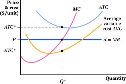
figure it out 8.2

For interactive, step-by-step help in solving the following problem, visit LaunchPad at http://www.macmillanhighered.com/launchpad/gls2e

Cardboard boxes are produced in a perfectly competitive market. Each identical firm has a short-run total cost curve of TC = 3Q³ – 18Q² + 30Q + 50, where Q is measured in thousands of boxes per week. The firm’s associated marginal cost curve is MC = 9Q² – 36Q + 30. Calculate the price below which a firm in the market will not produce any output in the short run (the shut-down price).

Solution:

A firm will not produce any output in the short run at any price below its minimum AVC. How do we find the minimum AVC? We learned in Chapter 7 that AVC is minimized when AVC = MC. So, we need to start by figuring out the equation for the average variable cost curve and then solving it for the output that minimizes AVC.

AVC is equal to VC/Q. Remember that total cost is the sum of fixed cost and variable cost:

TC = FC + VC

Fixed cost is that part of total cost that does not vary with output (changes in Q have no effect on FC). Therefore, if TC = 3Q³ – 18Q² + 30Q + 50, then FC must be 50. This means that VC = 3Q³ – 18Q² + 30Q. Because AVC = VC/Q,

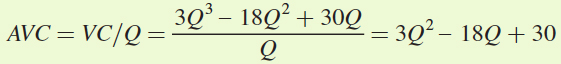
Next, we find the output for which AVC is at its minimum by equating AVC and MC:

AVC = MC

3Q² – 18Q + 30 = 9Q² – 36Q + 30

18Q = 6Q²

18 = 6Q

Q = 3

This means that AVC is at its minimum at an output of 3,000 cardboard boxes per week. To find the level of AVC at this output, we plug Q = 3 into the formula for AVC:

AVC = 3Q² – 18Q + 30

= 3(3)² – 18(3) + 30 = 27 – 54 + 30 = $3

Therefore, the minimum price at which the firm should operate is $3. If the price falls below $3, the firm should shut down in the short run and only pay its fixed cost.

298

make the grade

A tale of three curves

One of the easiest ways to examine the diagrams of cost curves for a perfectly competitive firm is to remember that each of these cost curves tells only a part of the story.

What is the profit-maximizing output? The marginal cost curve: If you want to know the level of output that maximizes profit for any firm, you need to use the firm’s marginal cost curve and equate marginal revenue and marginal cost. For a perfectly competitive firm only, you equate price and marginal cost because in perfect competition, marginal revenue is equal to price.

Is the firm earning a positive profit? The average total cost curve: Once you know the optimal level of output, you can use the average total cost curve to compare price and average total cost to determine whether a firm is earning a positive profit. Profit is measured as the rectangle with a base equal to output and a height equal to the difference between P and ATC at that quantity of output. If a perfectly competitive firm is earning a positive profit, the story ends there. You don’t even need to consider the firm’s average variable cost curve.

Operate or shut down? The average variable cost curve: If a firm is earning a loss (negative profit) because its price is less than its average total cost, the decision of whether or not the firm should continue to operate in the short run depends entirely on the relationship between price and average variable cost. Look at the average variable cost curve to determine how these two variables compare at the profit-maximizing/loss-minimizing level of output. If price is greater or equal, the firm should continue to operate; if average variable cost is greater, the firm should shut down.

Knowing which curve is used to answer these questions makes it easier to analyze complicated diagrams and answer questions for homework, quizzes, and exams. Remember that each curve has its own role and focus on that curve to simplify your analysis.

299