Most firms have some sort of market power, even if they are not monopolists. We recognized this reality in Chapter 8 when we noted that truly perfectly competitive firms are rare—farmers who grow commodity crops and maybe a few other firms take prices as completely given, but they’re the exception. The competitive market model is more of a useful starting point for studying market structures than it is a description of most product markets.

337

What does it mean, practically speaking, for a firm to have market power? Suppose BMW increased production of all its vehicle models by 5 times. We would expect the greater quantity of BMWs supplied to cause a movement down and along the demand curve to a new quantity at a lower price. Conversely, if BMW cut its production to one-fifth of its current level, we would expect BMW prices to rise. These outcomes mean that BMW should not act as if its production decisions don’t affect its prices. That is, BMW is not a price taker because the price of its product depends on the quantity of cars it produces. It faces a downward-sloping demand curve: If BMW produces more cars, it will drive down the market price. If it produces fewer cars, it will increase price.

In fact, because BMW doesn’t take its price as given, we could express the equivalent concept in terms of BMW choosing its price and letting the market determine the quantity it sells. That is, having market power means that if BMW sets a lower price for its cars, it will sell more of them, while if it raises prices, it will sell fewer. If a price-taking firm charges more than the market price, it will lose all its demand. But BMW won’t. This is exactly the idea introduced in our earlier discussion of Apple and the iPad. We can describe the firm’s decision in terms of either choosing its profit-maximizing price or choosing its profit-maximizing level of output; either way, we (and the firm) get the same result.

338

We made the argument that Apple was, effectively, a monopolist in the tablet computer market when it first introduced the iPad, but clearly we couldn’t say the same about BMW. It competes against several other automakers in every market in which it operates. Why, then, do we talk about its price-setting ability the same way we talk about Apple in the tablet computer market? We do so because the basic lessons of this chapter apply whenever a firm has any market power, even if it isn’t a monopolist. The key element of our analysis in this chapter is that a firm with market power faces a downward-sloping demand curve. In other words, its output level and price are interrelated. For a perfectly competitive firm, output level and price are not related. The market price (which it takes as given) is fixed and doesn’t change regardless of the quantity it sells. That is, a perfectly competitive firm’s demand curve is horizontal at the market-determined price.

True monopolies are not the only types of firms that have downward-sloping demand curves. They also exist in market structures in which firms face competitors. As we will see in Chapter 11, two common types of these other market structures are oligopoly, in which a few competitors operate in a market, and monopolistic competition, in which there are many firms in the market but each firm’s product is different enough that it faces a downward-sloping demand curve for the product it sells. The difference between monopoly and these other two cases is that in oligopoly and monopolistic competition, the particular shape of the demand curve faced by any given firm (even though it still slopes down) depends on the supply decisions of the other firms in the market. In a monopoly, however, there are no such interactions between firms, and so the firm’s demand curve is the market demand curve.

While we deal more extensively with the nature of interactions between firms in oligopoly and monopolistically competitive markets in Chapter 11, in this chapter, we analyze how a firm in those kinds of markets chooses its production (or price) level if other firms won’t change their behaviors in response to its choices. Having made this assumption, as long as the firm’s demand curve slopes downward, our analysis is the same whether this demand curve can be moved around by a competitor’s actions (as in an oligopoly or monopolistically competitive market) or not (as in a monopoly). As a result, we sometimes interchange the terms “market power” and “monopoly power” even if the firm we are analyzing is not literally a monopolist. The point is that once the firm’s demand curve is determined, its decision-making process is the same whether it is a monopoly, an oligopolistic firm, or a monopolistically competitive firm.2

The key to understanding how a firm with market power acts is to realize that, because it faces a downward-sloping demand curve, it can only sell more of its good by reducing its price. This one fact enters into every decision such firms make. As we learn later in the chapter, because firms with market power recognize the relationship between output and price, they will restrict output in a way that perfectly competitive firms won’t. They do so to keep prices higher (and thereby make more money).

339

To see why these firms restrict output to keep their prices high, we need to remember the concept of a company’s marginal revenue, the additional revenue a firm earns from selling one more unit. At first, that just sounds like the price of the product. And as we saw in Chapter 8, for a firm with no market power, this is exactly the case; the price is the marginal revenue. If a hotdog vendor walking the stands at a football game (a “firm” that can reasonably be thought of as a price taker) sells another hotdog, his total revenue goes up by whatever price he sells the hotdog for. The price doesn’t depend on how many hotdogs he sells; he is a price taker. He could sell hundreds of hotdogs and it wouldn’t change the market price, so his marginal revenue is just market price P.

But for a seller with market power, the concept of marginal revenue is more subtle. The extra revenue from selling another unit is no longer just the price. Yes, the firm can get the revenue from selling one more unit, but because the firm faces a downward-sloping demand curve, the more it chooses to sell, the lower the price will be for all units it sells, not just that one extra unit. (Important note: The firm is not allowed to charge different prices to different customers here. We deal with that scenario in Chapter 10.) This reduces the revenue the firm receives for the other units it sells. When computing the marginal revenue from selling that last unit, then, the firm must also subtract the loss it suffers on every other unit.

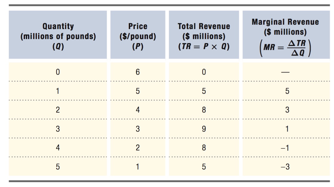
An example will clarify the firm’s situation. Let’s suppose that the firm in this case is Durkee-Mower, Inc., a Massachusetts firm that makes Marshmallow Fluff. Fluff has been around since 1920 and has a dominant position in the marshmallow creme market in the northeastern United States (you may have had some in a Fluffernutter sandwich, a s’more, or a Rice Krispies bar). This prominence in the market means that Durkee-Mower faces a downward-sloping demand curve for Fluff. If it makes more Fluff, its market price will fall, because the only way to get consumers to buy up the extra Fluff is to lower its price.

Table 9.1 shows how the quantity of Fluff produced this year varies with its price. As the quantity produced rises, the price falls because of the downward-sloping demand curve. The third column in Table 9.1 shows the total revenue for the year for each level of output. The marginal revenue of an additional unit of output (in this example, a unit is a million pounds) is shown in the last column. It equals the difference between total revenue at that level of output minus the total revenue had Durkee-Mower made one fewer unit.

340

If Durkee-Mower makes only 1 million pounds of Fluff, its price is $5 per pound, and its revenue is $5 million. Because total revenue would be zero if the firm didn’t produce anything, the marginal revenue of the first million pounds is $5 million. If Durkee-Mower makes 2 million pounds of Fluff instead, the market price falls to $4 per pound—the lower price makes consumers willing to buy another million pounds of Fluff. Total revenue in this case is $8 million. Therefore, the marginal revenue of increasing output from 1 to 2 million pounds is $3 million or $3 per pound. Note that this is less than the $4 per pound price that it sells for at the quantity of 2 million pounds.

As we discussed earlier, the lower marginal revenue reflects the fact that a firm with market power must reduce the price of its product when it produces more. Therefore, the marginal revenue isn’t just the price multiplied by the extra quantity, which would be ($4 per pound × 1 million pounds) = $4 million. It also subtracts the $1 million loss of revenue that occurs because the firm now sells the previous million units at a price that is $1 lower. Thus, the marginal revenue from producing 1 million more pounds of Fluff is $3 million: $4 million of revenue on the additional million pounds minus the $1 million lost from the price reduction on the initial million pounds sold.

If Durkee-Mower produces 3 million pounds, the market price drops to $3 per pound. Total revenue at this quantity is $9 million. The marginal revenue is now only $1 million. Again, this marginal revenue is less than the product of the market price and the extra quantity because producing more Fluff drives down the price that Durkee-Mower can charge for every unit it sells.

If the firm chooses to make still more Fluff, say, 4 million pounds, the market price drops further, to $2 per pound. Total revenue is now $8 million. That means in this case, Durkee-Mower has actually reduced its revenue (from $9 million to $8 million) by producing more Fluff, and marginal revenue is now negative (–$1 million). In this case, the price-drop revenue loss due to the extra production outweighs the revenue gains from selling more units. If Durkee-Mower insists on making 5 million pounds, the price drops to $1 per pound and total revenue falls to $5 million. Again, the marginal revenue of this million-pound unit is negative, –$3 million, because the revenue loss due to price reductions outweighs the extra units sold.

Why Does the Price Have to Fall for Every Unit the Firm Sells? One thing about marginal revenue that can be confusing for students at first glance is why the seller has to lower the price on all of its sales if it decides to produce one more unit. For instance, in the Marshmallow Fluff example, why can’t Durkee-Mower sell the first million pounds for $5 per pound, and then the second million pounds for $4 a pound, the third million for $3 a pound, and so on? That way the marginal revenue will always equal the price.

There are two reasons why the price drop applies to all units sold. The first is that we are not thinking of the firm’s decision as being sequential. Durkee-Mower isn’t deciding whether to sell a second million pounds after it has already sold its first million at $5 per pound. Instead, the firm is deciding whether to produce 1 million or 2 million pounds in this period. If it makes 1 million pounds, the price will be $5 per pound and revenue will be $5 million. If it instead produces 2 million pounds, each will be sold at a price of $4, and revenue will be $8 million. We are making the same assumption about the demand curve here that we have done throughout the book: The demand curve reflects demand during a given time period. All other issues of timing are ignored. Therefore, the demand curve reflects the quantity demanded in this period (a year in the Fluff example) at every price; whatever number of units the firm produces, they all sell at the same price.

The second reason why a price drop applies to all units sold is that we are assuming that, even within a particular time period, the market price has to be the same for all the units the firm sells. The firm can’t sell the first unit to a consumer who has a high willingness to pay and the second unit to a consumer with a slightly lower willingness to pay. This is probably a realistic assumption in many markets, including the market for marshmallow creme. Grocery stores don’t put multiple price tags on a given product. Imagine for a moment a scenario in which the price tag reads, “$5 if you really like Marshmallow Fluff, $4 if you like it but not quite as much, and $1 if you don’t really like Fluff but will buy it if it’s cheap.” In Chapter 10, we will look at situations where that sort of practice, called price discrimination, is possible.

341

Marginal Revenue: A Graphical ApproachThe idea that marginal revenue is different from the price is easy to see in a graph like Figure 9.1. On the downward-sloping demand curve, we can measure the total revenue TR (price × quantity) at two different points, x and y. At point x, the quantity sold is Q₁ and the price at which each unit is sold is P₁. The total revenue is price times quantity, seen in the figure as the rectangle A + B.

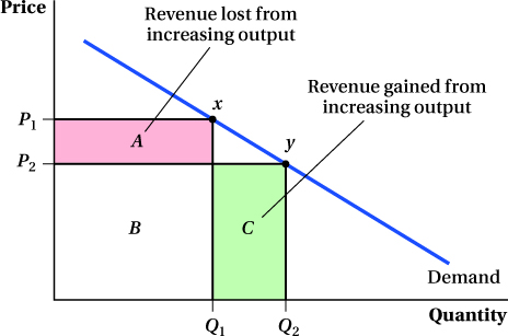
If the firm decides to produce more, say, by increasing output from Q₁ to Q₂, it will move to point y on the demand curve. The firm sells more units, but in doing so, the price falls to P₂. The new total revenue is P₂ × Q₂ or the rectangle B + C. Therefore, the marginal revenue of this output increase is the new revenue minus the old revenue:

TR₂ = P₂ × Q₂ = B + C

TR₁ = P₁ × Q₁ = A + B

MR = TR₂ – TR₁

MR = (B + C) – (A + B) = C – A

The area C contains the extra revenue that comes from selling more goods at price P₂, but this alone is not the marginal revenue of the extra output. We must also subtract area A, the revenue the firm loses because it now sells all units (not just the marginal unit) for the lower price P₂ instead of P₁. In fact, as we saw in the Fluff example, if the price-lowering effect of increasing output is large enough, it is possible that marginal revenue could be less than zero. In other words, selling more product could actually end up reducing a firm’s revenue.

Firms would like to engage in price discrimination if they could and sell different units at different prices, charging high willingness-to-pay consumers a high price and low willingness-to-pay consumers a low price, because they could avoid the loss in marginal revenue caused by price falling for all their sales. Again, we’re assuming that isn’t possible here, but in the next chapter, we will see what happens when they can.

342

Marginal Revenue: A Mathematical Approach We can compute a formula for a firm’s marginal revenue using the logic we just discussed. As we saw, there are two effects when the firm sells an additional unit of output. Each of these will account for a component of the marginal revenue formula.

The first effect comes from the additional unit being sold at the market price P. In Figure 9.1, if we define Q₂ – Q₁ to be 1 unit, then this effect would be area C.

The second effect occurs because the additional unit drives down the market price for all the units the firm makes. To figure out how to express this component of marginal revenue, let’s first label the change in price ΔP (so that, had the additional unit not been sold, the price would have been P + ΔP). In Figure 9.1, we’re looking at the effect of a decrease in price, so ΔP < 0. Let’s also label the quantity before adding the incremental unit of output as Q and the incremental output as ΔQ. The second component of marginal revenue is therefore the change in price caused by selling the additional unit of revenue times the quantity sold before adding the incremental unit. In Figure 9.1, this is area A. Note that because price falls as quantity rises—remember, the firm faces a downward-sloping demand curve—the term ΔP/ΔQ is negative. This conforms to our logic above that this second component of marginal revenue is negative. It is the loss in revenue resulting from having to sell the non-incremental units at a lower price.

Putting together these components, we have the formula for marginal revenue (MR) from producing an additional quantity (ΔQ) of output (notice that we add the two components together even though the second represents a loss in revenue because ΔP/ΔQ is already negative):

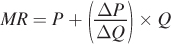
This negative second component means that marginal revenue will always be less than the market price. If we map this equation into Figure 9.1, the first term is the additional revenue from selling an additional unit at price P (area C) and the second is area A.

Looking more closely at this formula reveals how the shape of the demand curve facing a firm affects its marginal revenue. The change in price corresponding to a change in quantity, ΔP/ΔQ, is a measure of how steep the demand curve is. When the demand curve is really steep, price falls a lot in response to an increase in output. ΔP/ΔQ is a large negative number in this case. This will drive down MR and can even make it negative. On the other hand, when the demand curve is flatter, price is not very sensitive to quantity increases. In this case, because ΔP/ΔQ is fairly small in magnitude, the first (positive) component P of marginal revenue plays a larger relative role, keeping marginal revenue from falling too much as output rises. In the special case of perfectly flat demand curves, ΔP/ΔQ is zero, and therefore marginal revenue equals the market price of the good. We know from Chapter 8 that when a firm’s marginal revenue equals price, the firm is a price taker: Whatever quantity it sells will be sold at the market price P. This is an important insight that we return to below: Perfect competition is just the special case in which the firm’s demand curve is perfectly elastic, so MR = P.

This connection between the slope of the demand curve and the level of a firm’s marginal revenue is important in understanding how firms with market power choose the output levels that maximize their profits. We study this profit-maximization problem in detail in the next section, but it’s useful to reflect a bit now on what the marginal revenue formula implies about it. Firms that face steep demand curves obtain small revenue gains (or even revenue losses, if MR is negative) when they increase output. This makes high output levels less profitable. Firms facing flatter demand curves obtain relatively large marginal revenues when raising output. This contrast suggests that (holding all else equal) having a steeper demand curve tends to reduce a firm’s profit-maximizing output level. In the next section, we see that this is exactly the case.

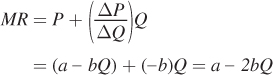
We can apply the marginal revenue formula to any demand curve. For nonlinear demand curves, the slope ΔP/ΔQ is the slope of a line tangent to the demand curve at quantity Q. But the formula is especially easy for linear demand curves, because ΔP/ΔQ is constant. For any linear (inverse) demand curve of the form P = a – bQ, where a (the vertical intercept of the demand curve) and b are constants, ΔP/ΔQ = –b. The inverse demand curve itself relates P (the other component of marginal revenue) to Q, so if we also plug P = a – bQ and ΔP/ΔQ = –b into the MR formula above, we arrive at an expression for the marginal revenue of any linear demand curve:

343

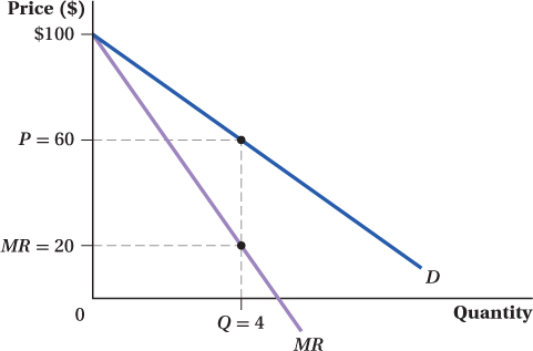
This formula shows that marginal revenue varies with the firm’s output. This is true in this specific case of a linear demand curve, but it’s important to recognize that it holds more generally. (The only exception to this outcome is for a perfectly competitive firm, for which marginal revenue is constant and equal to the market price for any production quantity.) Here, the marginal revenue curve looks a lot like the inverse demand curve. It has the same vertical intercept as the inverse demand curve, which is equal to a. (To see this, just plug Q = 0 into the demand and marginal revenue curves.) It also slopes down: A higher Q leads to lower marginal revenue. The only difference between the marginal revenue and demand curves is that the former is twice as steep: bQ in the inverse demand curve has been replaced with 2bQ. The formula for MR doesn’t just look like an inverse demand curve; it is conceptually similar, too. Just as the inverse demand curve shows how the price changes with production levels, the marginal revenue formula shows how marginal revenue changes with production levels. Further connecting the two curves is the fact that both the market price and marginal revenue are measured in the same units—dollars per unit of the good, for example.

An example of a demand curve and its marginal revenue curve is shown in Figure 9.2.3 The demand curve in the figure is P = 100 – 10Q and therefore the marginal revenue curve is MR = 100 – 20Q. If Q = 4, as shown, then the demand curve implies P = $60 and MR = $20.

344