20.1
MR-
Math Review Appendix
Section 1: Math Concepts and Basic Skills
There is no doubt that economics is about ideas. These economic ideas can be conveyed in a variety of languages—
Sometimes it’s easier to express and understand economic ideas using mathematical symbols rather than words. The material we present here reviews the algebra and geometry concepts we use in the text, as well as the calculus that the material in the appendices relies on. You have likely encountered most of these concepts and techniques before in your high school or college algebra or calculus classes, but we compile them here in a way that is most relevant to your study of economics. We will begin with a discussion of lines and curves, which are crucial to economic ideas such as utility and income, among others, and will set the foundation for the rest of our review.
Lines and Curves Functions describe the relationships between input variables and outputs, and may be written generically as y = f(x), where x is some input and y the output. One function crucial to our study is that of the line, which we commonly write in the form y=mx + b, and which we’ve graphed on the x-
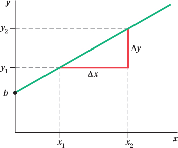
We can learn a lot from this functional form of the line, which is known as the slope-
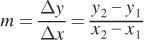
where Δ represents the change in a variable, and (x1, y1) and (x2, y2) are two points on the line.
MR-
The slope tells us two important pieces of information about the line. First, it describes how flat or steep the line is. In other words, we can answer the question: If x increases by one unit, by how much does y change? The slope also tells us whether the relationship between x and y is negative or positive. An upward-
The form y = mx + b holds one final piece of information about the line: b, or the y-intercept. You can clearly see this in Figure A.1—it’s where the line intersects the y-axis. In this case, the y-intercept is positive, but the line could also have a negative intercept and intersect the y-axis below the x-axis, or have a y-intercept equal to zero.1
1 A line may also have no y-intercept, although we won’t see these much in our study of intermediate microeconomics. This occurs when the line is vertical. Vertical lines will either intersect the y-axis at all points (if the line is equal to the y-axis, or x = 0) or, more commonly, not intersect the y-axis at all (say, for the line x = 2 or x = –4).
We have described the equation for the line using the slope-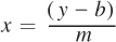 . In fact, we’ll see that last form a lot throughout our study of economics: It’s how we typically write supply and demand functions.
By definition, the slope of a straight line is constant; the slope will be the same no matter where you measure the change in x and y. But, the relationship between x and y may be more complicated. In contrast to the line, a curve can have different slopes at different points along it. Because a curve can have an almost infinite number of shapes and curvatures, there are no standard functional forms for curves.
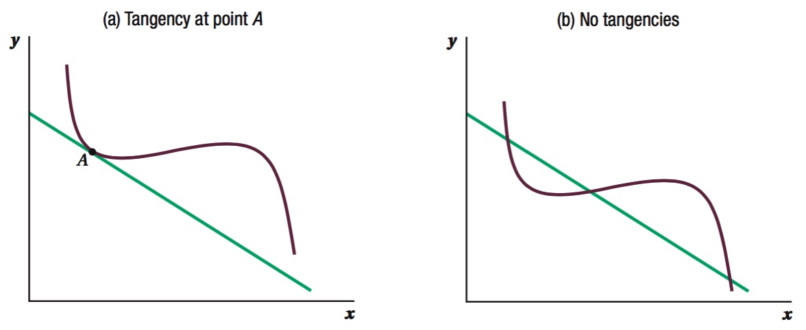
Tangency The point at which a given line and curve just touch—
Graphically, a tangent point is easy to see. Point A in panel a of Figure A.2 is a tangent point between the curve and a line. How can we tell this is a tangency? At A, the curve just touches the line without crossing it. In this case, this is the only point at which the slope of the curve equals the slope of the line, and is therefore tangent to the line.
MR-
figure it out A.1
A line has a slope of –2 and an intercept of 10.
Write the line in slope-
intercept form. Graph the line on a Cartesian plane.
Draw a curve tangent to the line.
Solution:
The slope-
intercept form of a line can be expressed as y = mx + b, where m is the slope and b is the intercept. The slope- intercept form corresponding to m = –2 and b = 10 therefore is y = –2x + 10. To graph the equation y = –2x + 10 on the Cartesian plane, we can calculate the coordinates of the intercepts and connect these points. Because the equation is in slope-
intercept form, we already know that the intercept along the y-axis occurs at point (0, 10). (Another way to solve for this is to plug x = 0 into the equation for the line. Note that when x = 0, y = –2(0) + 10 = 10.) To get the x-axis intercept, we can substitute y = 0 into the equation for the line: 0 = –2x + 10. Rearranging this equation, we see that 2x = 10 or x = 5. We therefore know that (5, 0) is another point along this line. Next, we connect these points to illustrate the line in the x-
y plane.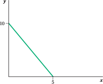
A curve tangent to the line y = –2x + 10 is included in the figure below. Note that, for this example, the tangency occurs at only one point on the line we graphed in the previous part of this problem. We could have drawn a curve that is tangent to the line at more than one point.
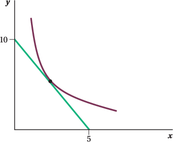
Not all lines and curves are tangent to each other. Panel b illustrates an example of a curve and a line that, while intersecting, have no tangencies.