The basic algebraic concepts we just reviewed are used throughout the book. We’ll turn now to calculus, which we use in the appendices to further our understanding of economic concepts. If you’ve taken calculus before, this section will be purely review. If you haven’t taken calculus, you might be able to pick up a few tricks. This section is not a substitute for a background in calculus. If you want to apply calculus to economics, it’s important to start with the solid foundation that an entry-level course in calculus provides.

MR-4

First Derivatives We have already seen that slopes are incredibly important to our study of economics. We can find the slope of a line using the formula . We had to stop short of describing the slope of a curve, since a curve’s slope, unlike that of a line, differs along the curve. This is where calculus can help us.

In particular, we can describe the slope of a curve (or a line) using a derivative, or the instantaneous rate of change of a function at a given point. Take the function y = f(x). Then we can write the derivative in the equivalent forms

Solving for first derivatives is easiest to demonstrate using examples of a few basic forms of derivatives, which we outline below. The rules we present are by no means an exhaustive list of derivatives rules. For that, you should consult a calculus text. But, these are the ones we’ll rely on in the calculus appendices, and which you’ll probably encounter most often in the context of economics.

Derivative of a constant: Take the function f(x) = c, where c is a constant. Then . Why? We know that a line of this form is horizontal at y = c. Since a horizontal line has a slope equal to zero, its derivative must also equal zero.

Power rule for derivatives: Perhaps the rule that we will most often rely on is the power rule. Given a function f(x) = cx^α, where c is again some constant as is the exponent α, the derivative takes the form . In words, you multiply x by its exponent and subtract one from the exponent you began with to find the derivative. This is perhaps best illustrated with an example. Take f(x) = 3x4. Then, .

Addition and subtraction rules for derivatives: We can rely on the rules above to find the derivatives for equations of the form f(x) = g(x) + h(x). To solve for , simply take the derivative of g(x) and h(x) separately:

As before, let’s illustrate this with a simple example. Take the function f(x) = x2 + 10. Then, .

Note that this rule applies whether you are adding or subtracting, since subtraction is simply the addition of a negative number. In other words, if .

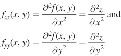
Second Derivatives We’ve found the derivative of a function, but sometimes we need to find the derivative of the derivative, or the second derivative:

What does the second derivative tell us about a function? While the first derivative describes the slope of a function, the second derivative describes a function’s curvature. A function’s curvature is said to be convex (as shown in Figure A.3, panel a) or concave (panel b). Note that a function may be convex over some values of x, and concave over others, such as in panel c.

MR-5

Over some range of x, a curve is said to be convex if the second derivative with respect to x is greater than zero, meaning that

It is concave when

These two rules we’ve presented may seem to be a bit of hand-waving, but the intuition behind them is clear. Consider first the meaning of a function’s first derivative: A positive (or negative) first derivative indicates that a function is increasing (or decreasing) over that region. Similarly then, the second derivative tells us whether the slope, as measured by its first derivative, is increasing or decreasing over that region. A positive second derivative indicates that the slope increases with higher values of x (panel a), which we call convexity; a negative second derivative means that the slope decreases with higher values of x (panel b), which we call concavity.2

2 Note that in panel a, the slope is increasing since it is becoming less negative as we move to the right. Similarly, the slope in panel b is decreasing since it is becoming more negative as we move to the right.

Partial Derivatives Above we found first and second derivatives for single-variable equations. Sometimes, however, we will need to find the slopes or curvatures of a multi-variable equation. In this case, we apply partial derivatives.

Consider the function z = f(x, y) where x and y are both inputs into the function that maps output z. Given this function, we can now find two partial first derivatives: the first derivative of z with respect to x, or and the first derivative of z with respect to y, or .

Calculating partial derivatives is actually quite simple when you know how to calculate a standard derivative. To find , you simply take the first derivative of f(x, y) with respect to x, holding y constant. Let’s demonstrate this with a standard Cobb–Douglas equation3 of the form f(x, y) = x^αy^1–α. Using the power rule for derivatives, we get

3 You will see Cobb–Douglas functions a lot in your study of economics—it is one of the most common functional forms for a variety of economics concepts, including utility and production functions. We won’t go into much detail about its properties here, but it is useful to see basic calculus techniques applied to this very common set of functions. In the calculus appendices, we’ll assume 0 < α < 1 for the purposes of solving economics problems. But to solve first and second partial derivatives, we don’t actually need to make this assumption, and so we don’t make it here. The exponent α could be negative or positive, fractional or a whole number, and the rules we present here still apply.

MR-6

Similarly,

These partial derivatives isolate the slopes (or rates of change of the function) in the x and y directions, respectively. What if we want to describe the curvatures of a multivariable function? To do this, we rely on second partial derivatives. It’s a bit of a tongue-twister, but it’s easiest to think about second partial derivatives in comparison to standard second derivatives: Second partial derivatives are partial derivatives of partial derivatives, just as standard second derivatives are standard derivatives of standard derivatives. For the function z = f(x, y), we are primarily interested in finding the curvature in two directions:

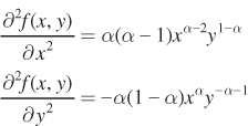
Using the Cobb–Douglas function from above, we get

There is actually, in this case, another type of second partial derivative that we could calculate. Known as a cross partial derivative, it calculates the first partial derivative with respect to x, and the second partial derivative with respect to y, or vice versa:

While it is useful to be aware of these cross partial derivatives, we will not rely on them for the analyses in this book.

One application of partial derivatives that we will use, however, is total differentiation. Total differentiation gives us the total change in a function, or the combined change in both the x and y directions. This comes up often in our study of economics: Sometimes we need to describe movements along a curve when two variables change simultaneously, as do a firm’s capital K and labor L inputs in Chapter 6. To totally differentiate a multi-variable function, we solve

Let’s break down what each part of this equation tells us. The two partial derivatives indicate the rate of change in the x and y directions, respectively. Likewise, dx and dy are the changes in x and y. Combining these as we do in the equation above gives us the total change of the function with respect to all variables.

MR-7

Unconstrained Optimization Problem In many ways, what we have been building up to in this math review is the last mathematical concept we will look at here: basic, or unconstrained, optimization. (For a consideration of constrained optimization, see the Appendix to Chapter 4.) In solving an optimization problem, we will rely on the derivative techniques we have learned thus far.

Begin with a function of the form y = f(x). We will first solve for what is known as the first-order condition. To do this, we set the first derivative equal to zero:

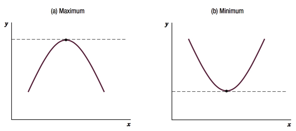
What does this tell us? Remember first that is the slope of the function f(x), examples of which are shown in Figure A.4. When this slope is zero, the line tangent to the curve is horizontal. This means that the curve must be at either a maximum (panel a) or a minimum (panel b).

We actually don’t yet know whether the first-order condition we found has given us a maximum or a minimum. We just know that we have found an optimum. To learn whether we have maximized or minimized the function, we need to return to our second piece of derivative knowledge: second derivatives. Specifically, we need to take the second derivative of the function, and test whether it is negative or positive:

When , the curve is concave, and the point is a maximum.

When , the curve is convex, and the point is a minimum.

MR-8