Research Methods Used by Psychologists

Regardless of their perspective, psychology researchers use the same research methods. These methods fall into three categories—descriptive, correlational, and experimental. The experimental method is used most often because it allows the researcher to explore cause–effect relationships. Remember, the main goal of psychology is to explain (through cause–effect relationships) human behavior and mental processes. However, sometimes researchers can't conduct experiments. For example, it is obviously unethical to set up an experiment testing the effects of passive smoking on children. Who would knowingly subject a group of children to cigarette smoke? In such situations, psychologists can learn a lot by employing the other methods—descriptive and correlational. Researchers can carefully observe and describe the health effects on one child in a family of smokers, or they can study many families in search of relationships (correlations) between parental smoking and childhood infections. These other research methods also provide data for developing hypotheses (testable predictions about cause–effect relationships) to examine in experimental research. We'll discuss the three types of methods in the following order: descriptive, correlational, and experimental.

Descriptive Methods

There are three types of descriptive methods: observational techniques, case studies, and survey research. The main purpose of all three methods is to provide objective and detailed descriptions of behavior and mental processes. However, these descriptive data only allow the researcher to speculate about cause–effect relationships—to develop hypotheses about causal relationships. Such hypotheses must then be tested in experiments. With this important limitation in mind, we'll consider the three descriptive methods one at a time.

Observational techniques.

Observational techniques exactly reflect their name. The researcher directly observes the behavior of interest. Such observation can be done in the laboratory. For example, children's behavior can be observed using one-way mirrors in the laboratory. However, behavior in the laboratory setting may not be natural. This is why researchers often use naturalistic observation, a descriptive research method in which behavior is observed in its natural setting, without the researcher intervening in the behavior being observed. Researchers use naturalistic observation when they are interested in how humans or other animals behave in their natural environments. The researcher attempts to describe both objectively and thoroughly the behaviors that are present and the relationships among these behaviors. There have been many well-known observational studies of other species of animals in their natural habitats. You are probably familiar with some of them—Dian Fossey's study of mountain gorillas in Africa, on which the movie, Gorillas in the Mist, was based, and Jane Goodall's study of chimpanzees in Africa (Fossey, 1983; Goodall, 1986). This method is not used only for the observation of other species of animals. Observational studies of human behavior are conducted in many natural settings such as the workplace and school and in social settings such as bars.

Lady studying chimps, chimp studying lady.

cartoonstock

Observational techniques do have a major potential problem, though. The observer may influence or change the behavior of those being observed. This is why observers must remain as unobtrusive as possible, so that the results won't be contaminated by their presence. To overcome this possible shortcoming, researchers use participant observation. In participant observation, the observer becomes part of the group being observed. Sometimes naturalistic observation studies that start out with unobtrusive observation end up as participant observation studies. For example, Dian Fossey's study of gorillas turned into participant observation when she was finally accepted as a member of the group. However, in most participant observation studies, the observer begins the study as a participant, whether in a laboratory or natural setting. You can think of this type of study as comparable to doing undercover work. A famous example of such a study involved a group of people posing as patients with symptoms of a major mental disorder to see if doctors at psychiatric hospitals could distinguish them from real patients (Rosenhan, 1973). It turned out that the doctors couldn't do so, but the patients could. Once admitted, these “pseudopatients” acted normally and asked to be released to see what would happen. Well, they weren't released right away. We will find out what happened to them in Chapter 10.

Case studies.

Detailed observation is also involved in a case study. In a case study, the researcher studies an individual in depth over an extended period of time. In brief, the researcher attempts to learn as much as possible about the individual being studied. A life history for the individual is developed, and data for a variety of tests are collected. The most common use of case studies is in clinical settings with patients suffering specific deficits or problems. The main goal of a case study is to gather information that will help in the treatment of the patient. The results of a case study cannot be generalized to the entire population. They are specific to the individual that has been studied. However, case study data do allow researchers to develop hypotheses that can then be tested in experimental research. A famous example of such a case study is that of the late Henry Molaison, a person with amnesia (Scoville & Milner, 1957). He was studied by nearly 100 investigators (Corkin, 2002) and is often referred to as the most studied individual in the history of neuroscience (Squire, 2009). For confidentiality purposes while he was alive (he died in 2008 at the age of 82), only his initials, H. M., were used to identify him in the hundreds of studies that he participated in for over five decades. Thus, we will refer to him as H. M. His case will be discussed in more detail in Chapter 5 (Memory), but let's consider some of his story here to illustrate the importance of case studies in the development of hypotheses and the subsequent experimental work to test these hypotheses.

For medical reasons, H. M. had his hippocampus (a part of the brain below the cortex) and the surrounding areas surgically removed at a young age. His case study included testing his memory capabilities in depth after the operation. Except for some amnesia for a period preceding his surgery (especially events in the days immediately before the surgery), he appeared to have normal memory for information that he had learned before the operation, but he didn't seem to be able to form any new memories. For example, if he didn't know you before his operation, he would never be able to remember your name regardless of how many times you met with him. He could read a magazine over and over again without ever realizing that he had read it before. He couldn't remember what he had eaten for breakfast. Such memory deficits led to the hypothesis that the hippocampus plays an important role in the formation of new memories; later experimental research confirmed this hypothesis (Cohen & Eichenbaum, 1993). We will learn exactly what role the hippocampus plays in memory in Chapter 5. Remember, researchers cannot make cause–effect statements based on the findings of a case study, but they can formulate hypotheses that can be tested in experiments.

Survey research.

The last descriptive method is one that you are most likely already familiar with, survey research. You have probably completed surveys either online, over the phone, via the mail, or in person during an interview. Survey research uses questionnaires and interviews to collect information about the behavior, beliefs, and attitudes of particular groups of people. It is assumed in survey research that people are willing and able to answer the survey questions accurately. However, the wording, order, and structure of the survey questions may lead the participants to give biased answers (Schwartz, 1999). For example, survey researchers need to be aware of the social desirability bias, our tendency to respond in socially approved ways that may not reflect what we actually think or do. This means that questions need to be constructed carefully to minimize such biases. Developing a well-structured, unbiased set of survey questions is a difficult, time-consuming task, but one that is essential to doing good survey research.

“Next question: I believe that life is a constant striving for balance, requiring frequent tradeoffs between morality and necessity, within a cyclic pattern of joy and sadness, forging a trail of bittersweet memories until one slips, inevitably, into the jaws of death. Agree or disagree?”

George Price/The New Yorker Collection/www.cartoonbank.com

Another necessity in survey research is surveying a representative sample of the relevant population, the entire group of people being studied. For many reasons (such as time and money), it is impossible to survey every person in the population. This is why the researcher only surveys a sample, the subset of people in a population participating in a study. For these sample data to be meaningful, the sample has to be representative of the larger relevant population. If you don't have a representative sample, then generalization of the survey findings to the population is not possible.

One ill-fated survey study of women and love (Hite, 1987) tried to generalize from a nonrepresentative sample (Jackson, 2012). Shere Hite's sample was drawn mainly from women's organizations and political groups, plus some women who requested and completed a survey following the researcher's talk-show appearances. Because such a sample is not representative of American women in general, the results were not either. For example, the estimates of the numbers of women having affairs and disenchanted in their relationships with men were greatly overestimated. To obtain a representative sample, survey researchers usually use random sampling.

In random sampling, each individual in the population has an equal opportunity of being in the sample. To understand the “equal opportunity” part of the definition, think about selecting names from a hat, where each name has an equal opportunity for being selected. In actuality, statisticians have developed procedures for obtaining a random sample that parallel selecting names randomly from a hat. Think about how you would obtain a random sample of first-year students at your college. You couldn't just sample randomly from those first-year students in your psychology class. All first-year students wouldn't have an equal opportunity to be in your sample. You would have to get a complete list of all first-year students from the registrar and then sample randomly from it. The point to remember is that a survey study must have a representative sample in order to generalize the research findings to the population.

Correlational Studies

In a correlational study, two variables are measured to determine if they are related (how well either one predicts the other). A variable is any factor that can take on more than one value. For example, age, height, grade point average, and intelligence test scores are all variables. In conducting a correlational study, the researcher first gets a representative sample of the relevant population. Next, the researcher takes the two measurements on the sample. For example, the researcher could measure a person's height and their weight.

The correlation coefficient.

To see if the variables are related, the researcher calculates a statistic called the correlation coefficient, a statistic that tells us the type and the strength of the relationship between two variables. Correlation coefficients range in value from -1.0 to +1.0. The sign of the coefficient, + or -, tells us the type of relationship, positive or negative. A positive correlation indicates a direct relationship between two variables—low scores on one variable tend to be paired with low scores on the other variable, and high scores on one variable tend to be paired with high scores on the other variable. Think about the relationship between height and weight. These two variables are positively related. Taller people tend to be heavier. SAT scores and first-year college grades are also positively correlated (Linn, 1982). Students who have higher SAT scores tend to get higher grades during their first year of college.

A negative correlation is an inverse relationship between two variables—low scores on one variable tend to be paired with high scores on the other variable, and high scores on one variable tend to be paired with low scores on the other variable. A good example of a negative correlation is the relationship for children between time spent watching television and grades in school—the more time spent watching television, the lower the school grades (Ridley-Johnson, Cooper, & Chance, 1983). As you know if you have ever climbed a mountain, elevation and temperature are negatively correlated—as elevation increases, temperature decreases. In summary, the sign of the coefficient tells us the type of the relationship between the two variables—positive (+) for a direct relationship or negative (-) for an inverse relationship.

The second part of the correlation coefficient is its absolute value, from 0 to 1.0. The strength of the correlation is indicated by its absolute value. Zero and absolute values near zero indicate no relationship. As the absolute value increases to 1.0, the strength of the relationship increases. Please note that the sign of the coefficient does not tell us anything about the strength of the relationship. Coefficients do not function like numbers on the number line, where positive numbers are greater than negative numbers. With correlation coefficients, only the absolute value of the number tells us about the relationship's strength. For example, -.50 indicates a stronger relationship than +.25. As the strength of the correlation increases, researchers can predict the relationship with more accuracy. If the coefficient is + (or -) 1.0, we have perfect predictability. A correlation of (+or -) 1.0 means that every change in one variable is accompanied by an equivalent change in the other variable in the same direction. Virtually all correlation coefficients in psychological research have an absolute value less than 1.0. Thus, we usually do not have perfect predictability so there will be exceptions to these relationships, even the strong ones. These exceptions do not, however, invalidate the general trends indicated by the correlations. They only indicate that the relationships are not perfect. Because the correlations are not perfect, such exceptions have to exist.

Scatterplots.

A good way to understand the predictability of a coefficient is to examine a scatterplot—a visual depiction of correlational data. In a scatterplot, each data point represents the scores on the two variables for each participant. Several sample scatterplots are presented in Figure 1.1. Correlational studies usually involve a large number of participants; therefore there are usually a large number of data points in a scatterplot. Because those in Figure 1.1 are just examples to illustrate how to interpret scatterplots, there are only 15 points in each one. This means there were 15 participants in each of the hypothetical correlational studies leading to these scatterplots.

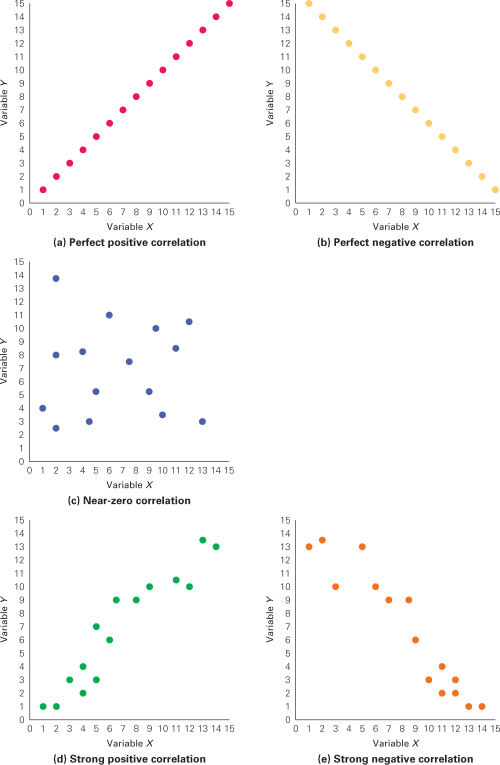
Figure 1.1 Some Sample Scatterplots (a) and (b) are examples of perfect correlations because there is no scatter—all of the data points in each plot fall on the same line. The correlation in (a) is positive because the data points show an increasing trend (go from bottom left to top right) and is negative in (b) because the data points show a decreasing trend (go from top left to bottom right). (c) is an example of a near-zero correlation because the data points are scattered all over and do not show a directional trend. (d) is an example of a strong positive correlation because there is not much scatter and the data points have an increasing trend. (e) is an example of a strong negative correlation because there is not much scatter and the data points show a decreasing trend.

The scatterplots in Figure 1.1(a) and Figure 1.1(b) indicate perfect 1.0 correlations—(a) a perfect positive correlation and (b) a perfect negative correlation. All of the points fall on the same line in each scatterplot, which allows us to predict one variable from the other perfectly by using the equation for the line. This means that you have maximal predictability. Please note that the difference between (a) and (b) is the direction of the data points (line). If the data points show an increasing trend (go from the bottom left to the top right of the scatterplot) as in (a), it is a positive relationship. Low scores on one variable tend to be paired with low scores on the other variable, and high scores with high scores. This is a direct relationship. However, if the data points show a decreasing trend (go from the top left to the bottom right) as in (b), there is a negative relationship. Low scores tend to be paired with high scores, and high scores with low scores. This is an inverse relationship.

The scatterplot in Figure 1.1(c) indicates no relationship between the two variables. There is no direction to the data points in this scatterplot. They are scattered all over in a random fashion. This means that we have a correlation near 0 and minimal predictability. Now consider (d) and (e). First, you should realize that (d) indicates a positive correlation because of the direction of the data points from the bottom left to the top right and that (e) indicates a negative correlation because of the direction of the scatter from the top left to the bottom right. But what else does the scatter of the data points tell us? Note that the data points in (d) and (e) neither fall on the same line as in (a) and (b), nor are they scattered all about the graph with no directional component as in (c). Thus, scatterplots (d) and (e) indicate correlations with strengths somewhere between 0 and 1.0. As the amount of scatter of the data points increases, the strength of the correlation decreases. So, how strong would the correlations represented in (d) and (e) be? They would be fairly strong because there is not much scatter. Remember, as the amount of scatter increases, the strength decreases and so does predictability. When the scatter is maximal as in (c), the strength is near 0, and we have little predictability.

The third-variable problem.

correlations give us excellent predictability, but they do not allow us to draw cause–effect conclusions about the relationships between the variables. I cannot stress this point enough. Correlation is necessary but not sufficient for causation to exist. Remember, correlational data do not allow us to conclude anything about cause–effect relationships. Only data collected in well-controlled experiments allow us to draw such conclusions. This does not mean that two correlated variables cannot be causally related, but rather that we cannot determine this from correlational data. Maybe they are; maybe they are not. Correlational data do not allow you to decide if they are or are not. Let's see why.

DILBERT © 2011 Scott Adams. Used By permission of UNIVERSAL UCLICK. All rights reserved

To understand this point, let's consider the negative correlation between self-esteem and depression. As self-esteem decreases, depression increases. But we cannot conclude that low self-esteem causes depression. First, it could be the reverse causal relationship. Isn't it just as likely that depression causes low self-esteem? Second, and of more consequence, isn't it possible that some third factor is responsible for the relationship between the two variables? For example, isn't it possible that some people have a biological predisposition for both low self-esteem and depression or that both self-esteem and depression are the result of a brain chemistry problem? Both self-esteem and depression could also stem from some current very stressful events. Such alternative possibilities are examples of the third-variable problem—another variable may be responsible for the relationship observed between two variables. In brief, such “third variables” are not controlled in a correlational study, making it impossible to determine the cause for the observed relationship.

To make sure you understand the third-variable problem, here is a very memorable example (Li, 1975, described in Stanovich, 2004). Because of overpopulation problems, a correlational study was conducted in Taiwan to identify variables that best predicted the use of contraceptive devices. Correlational data were collected on many different variables, but the researchers found that use of contraceptive devices was most strongly correlated with the number of electrical appliances in the home! Obviously having electrical appliances such as television sets, microwave ovens, and toasters around does not cause people to use birth control. What third variable might be responsible for this relationship? Think about it. A likely one is level of education. People with a higher education tend to be both better informed about birth control and to have a higher socioeconomic status. The former leads them to use contraceptive devices, and the latter allows them to buy more electrical appliances. Whelan (2013) describes a similar example of the third-variable problem in his book Naked Statistics. Consider the positive correlation between a student's SAT scores and the number of television sets that his family owns. Obviously this does not mean that parents can boost their children's test scores by buying another half-dozen television sets. Nor does it likely mean that watching lots of television is good for academic achievement (we have already learned that it isn't). The most logical explanation would be that highly educated people can afford a lot of television sets and tend to have children who test better than average. Both the number of television sets and the test scores are likely the result of a third variable, parental education. To control for the effects of such third variables, researchers conduct an experiment in which they manipulate one variable and measure its effect upon another variable while controlling other potentially relevant variables. Researchers must control for possible third variables so that they can make cause–effect statements. Such control, manipulation, and measurement are the main elements of experimental research, which is described next.

Experimental Research

The key aspect of experimental research is that the researcher controls the experimental setting. The only factor that varies is what the researcher manipulates. It is this control that allows the researcher to make cause–effect statements about the experimental results. This control is derived primarily from two actions. First, the experimenter controls for the possible influence of third variables by making sure that they are held constant across all of the groups or conditions in the experiment. Second, the experimenter controls for any possible influences due to the individual characteristics of the participants, such as intelligence, motivation, and memory, by using random assignment—randomly assigning the participants to groups in an experiment in order to equalize participant characteristics across the various groups in the experiment. If the participant characteristics of the groups are on average equivalent at the beginning of the experiment, then any differences between the groups at the end of the experiment cannot be attributed to such characteristics.

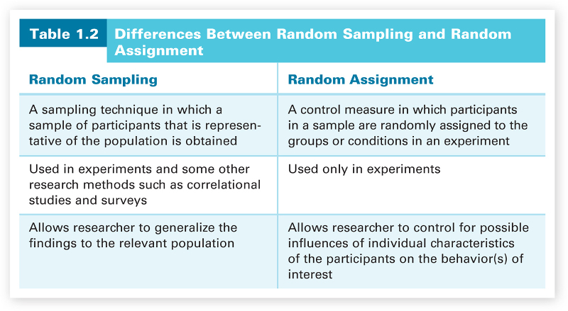
Please note the differences between random assignment and random sampling. Random sampling is a technique in which a sample of participants that is representative of a population is obtained. Hence it is used not only in experiments but also in other research methods such as correlational studies and surveys. Random assignment is only used in experiments. It is a control measure in which the researcher randomly assigns the participants in the sample to the various groups or conditions in an experiment. Random sampling allows you to generalize your results to the relevant population; random assignment controls for possible influences of individual characteristics of the participants on the behavior(s) of interest in an experiment. These differences between random sampling and random assignment are summarized in Table 1.2.

Designing an experiment.

When a researcher designs an experiment, the researcher begins with a hypothesis (the prediction to be tested) about the cause–effect relationship between two variables. One of the two variables is assumed to be the cause, and the other variable is the one to be affected. The independent variable is the hypothesized cause, and the experimenter manipulates it. The dependent variable is the variable that is hypothesized to be affected by the independent variable and thus is measured by the experimenter. Thus, in an experiment the researcher manipulates the independent variable and measures its effect on the dependent variable while controlling other potentially relevant variables. If there is a causal relationship between the independent and dependent variables, then the measurements of the dependent variable are dependent on the values of the independent variable, hence the name dependent variable. Sometimes the researcher hypothesizes more than one cause or more than one effect so he manipulates more than one independent variable or measures more than one dependent variable. To help you understand this terminology and the mechanics of an experiment, I'll describe an example.

Let's consider the simplest experiment first—only two groups. For control purposes, participants are randomly assigned to these two groups. One of the groups will be exposed to the independent variable, and the other will not. The group exposed to the independent variable is called the experimental group, and the group not exposed to the independent variable is called the control group. Let's say the experimenter's hypothesis is that aerobic exercise reduces anxiety. The independent variable that will be manipulated is aerobic exercise, and the dependent variable that will be measured is level of anxiety. The experimental group will participate in some aerobic exercise program, and the control group will not. To measure any possible effects of the aerobic exercise on anxiety, the experimenter must measure the anxiety levels of the participants in each group at the beginning of the study before the independent variable is manipulated, and then again after the manipulation. If the two groups are truly equivalent, the level of anxiety for each group at the beginning of the study should be essentially the same. If the aerobic exercise does reduce anxiety, then we should see this difference in the second measurement of anxiety at the end of the experiment.

The independent and dependent variables in an experiment must be operationally defined. An operational definition is a description of the operations or procedures the researcher uses to manipulate or measure a variable. In our sample experiment, the operational definition of aerobic exercise would include the type and the duration of the activity. For level of anxiety, the operational definition would describe the way the anxiety variable was measured (for example, a participant's score on a specified anxiety scale). Operational definitions not only clarify a particular experimenter's definitions of variables but also allow other experimenters to attempt to replicate the experiment more easily, and replication is the cornerstone of science (Moonesinghe, Khoury, & Janssens, 2007).

Let's go back to our aerobic exercise experiment. We have our experimental group and our control group, but this experiment really requires a second control group. The first control group (the group not participating in the aerobic exercise program) provides a baseline level of anxiety to which the anxiety of the experimental group can then be compared. In other words, it controls for changes in the level of anxiety not due to aerobic exercise. However, we also need to control for what is called the placebo effect—improvement due to the expectation of improving because of receiving treatment. The treatment involved in the placebo effect, however, only involves receiving a placebo—an inactive pill or a treatment that has no known effects. The placebo effect can arise not only from a conscious belief in the treatment but also from subconscious associations between recovery and the experience of being treated (Niemi, 2009). For example, stimuli that a patient links with getting better, such as a doctor's white lab coat or the smell of an examining room, may induce some improvement in the patient's condition. In addition, giving a placebo a popular medication brand name, prescribing more frequent doses, using placebo injections rather than pills, or indicating that it is expensive can boost the effect of a placebo (Niemi, 2009; Stewart-Williams, 2004; Waber, Shiv, Carmon, & Ariely, 2008). Recent research has even found that the placebo effect may not require concealment or deception (Kaptchuk et al., 2010Ƒ and, in the case of pain, that it's size may be impacted by personality traits, such as altruism and resilience (Peciña et al., 2013).

from Mordantorange.com, Mike Bannon, cartoonist

The placebo (Latin for “I will please) effect, however, does have an evil twin, the nocebo (Latin for “I will harm”) effect, whereby expectation of a negative outcome due to treatment leads to adverse effects (Benedetti, Lanotte, Lopiano, & Colloca, 2007; Kennedy 1961). Thus, expectations can also do harm; hence, the nocebo effect is sometimes referred to as a negative placebo effect. For example, when a patient anticipates a drug's possible side effects, he can suffer them even if the drug is a placebo. Because of ethical reasons, the nocebo effect has not been studied nearly as much as the placebo effect, but recently Häuser, Hansen, and Enck (2012) reviewed 31 studies that clearly demonstrated the nocebo effect in clinical practice. They concluded that the nocebo effect creates an ethical dilemma for physicians and therapists—how to fully inform patients of the potential complications of treatment and at the same time minimize inducing these complications through nocebo effects. Thus, research on the nocebo effect has mainly centered on its critical role in clinical practice whereas much of the research on the placebo effect has been concerned with controlling for improvement due to participant expectations, as in our aerobic exercise experiment.

The reduction of anxiety in the experimental group participants in our aerobic exercise experiment may be partially or completely due to a placebo effect. This is why researchers add a control group called the placebo group to control for the possible placebo effect. A placebo group is a group of participants who believe they are receiving treatment, but they are not. They get a placebo. For example, the participants in a placebo group in the aerobic exercise experiment would be told that they are getting an antianxiety drug, but they would only get a placebo (in this case, a pill that has no active ingredient). The complete design for the aerobic exercise experiment, including the experimental, placebo, and control groups, is shown in Figure 1.2. For the experimenter to conclude that there is a placebo effect, the reduction of anxiety in the placebo group would have to be significantly greater than the reduction for the control group. For the experimenter to conclude that the reduction of anxiety in the experimental group is due to aerobic exercise and not a placebo effect, it would have to be significantly greater than that observed for the placebo group.

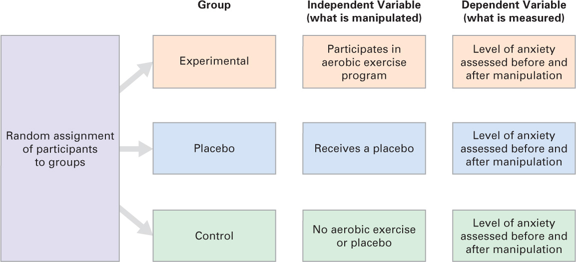Figure 1.2 Design of Aerobic Exercise and Anxiety Experiment Participants are randomly assigned to groups in order to equalize participant characteristics across the groups. The placebo group controls for the placebo effect, and the control group provides a baseline level of anxiety reduction for participants who do not participate in the aerobic exercise program or receive a placebo. The level of anxiety reduction for each group is determined by comparing the measurements of the dependent variable (level of anxiety) before and after manipulating the independent variable (aerobic exercise).

Now you may be wondering what is meant by “significantly greater.” This is where statistical analysis enters the scene. We use what are called inferential statistical analyses—statistical analyses that allow researchers to draw conclusions about the results of their studies. Such analyses tell the researcher the probability that the results of the study are due to random variation (chance). Obviously, the experimenter would want this probability to be low. Remember, the experimenter's hypothesis is that the manipulation of the independent variable (not chance) is what causes the dependent variable to change. In statistics, a “significant” finding is one that has a probability of .05 (1/20) or less that it is due to chance. Thus, a significant finding is one that is probably not due to chance.

Statistical significance tells us that a result probably did not occur by chance, but it does not insure that the finding has practical significance or value in our everyday world. A statistically significant finding with little practical value sometimes occurs when very large samples are used in a study. With such samples, very small differences among groups may be significant. Belmont and Marolla's (1973) finding of a birth-order effect for intelligence test scores is a good example of such a finding. Belmont and Marolla analyzed intelligence test data for almost 400,000 19-year-old Dutch males. There was a clear birth-order effect: First borns scored significantly higher than second borns, second borns higher than third borns, and so on. However, the score difference between these groups was very small (only a point or two) and thus not of much practical value. So remember, statistically significant findings do not always have practical significance.

“It was more of a ‘triple-blind’ test. The patients didn't know which ones were getting the real drug, the doctors didn't know, and I'm afraid, nobody knew.”

1996 Sidney Harris

The aerobic exercise experiment would also need to include another control measure, the double-blind procedure. In the double-blind procedure, neither the experimenters nor the participants know which participants are in the experimental and control groups. This procedure is called “double-blind” because both the experimenters and participants are blind to (do not know) the participant group assignments. It is not unusual for participants to be blind to which group they have been assigned. This is especially critical for the placebo group participants. If they were told that they were getting a placebo, there would be no expectation for getting better and hence no (or a much reduced) placebo effect. But why should the experimenters not know the group assignments of the participants? This is to control for the effects of experimenter expectation (Rosenthal, 1966, 1994). If the experimenters knew which condition the participants were in, they might unintentionally treat them differently and thereby affect their behavior. In addition, the experimenters might interpret and record the behavior of the participants differently if they needed to make judgments about their behavior (their anxiety level in the example study). The key for the participant assignments to groups is kept by a third party and then given to the experimenters once the study has been conducted.

Now let's think about experiments that are more complex than our sample experiment with its one independent variable (aerobic exercise) and two control groups. In most experiments, the researcher examines multiple values of the independent variable. With respect to the aerobic exercise variable, the experimenter might examine the effects of different amounts or different types of aerobic exercise. Such manipulations would provide more detailed information about the effects of aerobic exercise on anxiety. An experimenter might also manipulate more than one independent variable. For example, an experimenter might manipulate diet as well as aerobic exercise. Different diets (high-protein vs. high-carbohydrate diets) might affect a person's level of anxiety in different ways. The two independent variables (diet and aerobic exercise) might also interact to determine one's level of anxiety. An experimenter could also increase the number of dependent variables. For example, both level of anxiety and level of depression could be measured in our sample experiment, even if only aerobic exercise were manipulated. If aerobic exercise reduces anxiety, then it might also reduce depression. As an experimenter increases the number of values of an independent variable, the number of independent variables, or the number of dependent variables, the possible gain in knowledge about the relationship between the variables also increases. Thus, most experiments are more complex in design than our simple example with an experimental group and two control groups. In addition, many experimental studies, including replications, must be conducted to address any experimental question. Researchers have a statistical technique called meta-analysis that combines the results for a large number of studies on one experimental question into one analysis to arrive at an overall conclusion. Because a meta-analysis involves the results of numerous experimental studies, its conclusion is considered much stronger evidence than the results of an individual study in answering an experimental question.

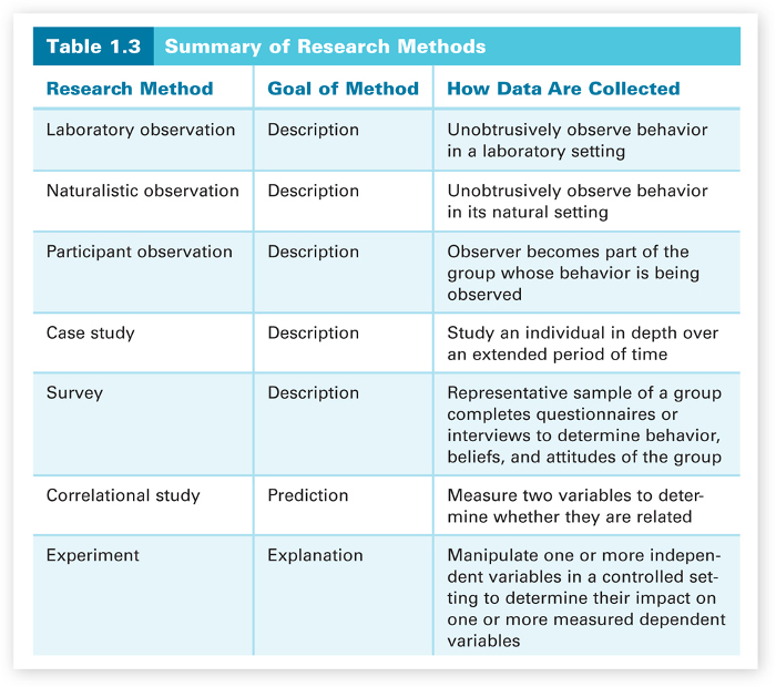
The various research methods that have been discussed are summarized in Table 1.3. Their purposes and data-gathering procedures are described. Make sure you understand each of these research methods before going on to the next section, where we'll discuss how to understand research results. If you feel that you don't understand a particular method, go back and reread the information about it until you do.