Learning Through Operant Conditioning

In the previous section, we described classical conditioning—learning about associations between stimuli in our environment. In this section, we will consider another important type of conditioning, operant conditioning—learning to associate behaviors with their consequences. Behaviors that are reinforced (lead to satisfying consequences) will be strengthened, and behaviors that are punished (lead to unsatisfying consequences) will be weakened. The behavior that is reinforced or punished is referred to as the operant response because it “operates” on the environment by bringing about certain consequences. We are constantly “operating” on our environment and learning from the consequences of our behavior. For example, in meeting someone whom you like and want to date, your behavior (what you say and how you act) will either lead to satisfying consequences (a date) or unsatisfying consequences (no date). Satisfying consequences will lead you to act that way again in the future; unsatisfying consequences will lead you to change your behavior.

Edward Thorndike used puzzle boxes like the functional representation shown here in his classic learning studies with cats. The boxes varied in how difficult they were for the cats to escape from. The illustration shows one of the easier boxes—pulling on a looped string raised the bolt to open the door. More difficult boxes required the cat to make more than one response. The results of these puzzle box experiments led Thorndike to develop the law of effect.

Science Source

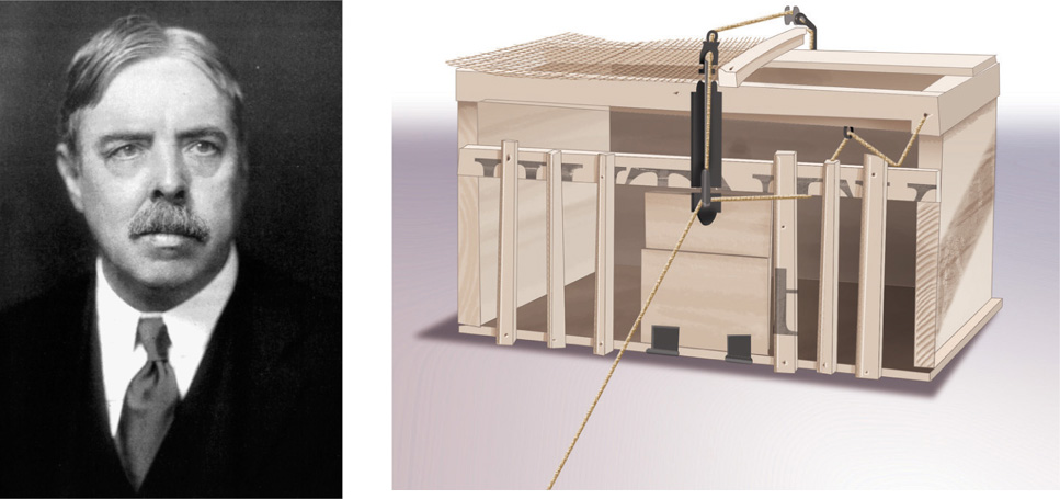
Research on how we learn associations between behaviors and their consequences started around the beginning of the twentieth century. American psychologist Edward Thorndike studied the ability of cats and other animals to learn to escape from puzzle boxes (Thorndike, 1898, 1911). In these puzzle boxes, there was usually only one way to get out (for example, pressing a lever would open the door). Thorndike would put a hungry animal in the box, place food outside the box (but in sight of the animal), and then record the animal’s behavior. If the animal pressed the lever, as a result of its behavior it would manage to escape the box and get the food (satisfying effects). The animal would tend to repeat such successful behaviors in the future when put back into the box. However, other behaviors (for example, pushing the door) that did not lead to escaping and getting the food would not be repeated.

Based on the results of these puzzle box experiments, Thorndike developed what he termed the law of effect—any behavior that results in satisfying consequences tends to be repeated, and any behavior that results in unsatisfying consequences tends not to be repeated. In the 1930s, B. F. (Burrhus Frederic) Skinner, the most influential of all behaviorists, redefined the law in more objective terms and started the scientific examination of how we learn through operant conditioning (Skinner, 1938). Let’s move on to Skinner’s redefinition and a description of how operant conditioning works.

Learning Through Reinforcement and Punishment

To understand how operant conditioning works, we first need to learn Skinner’s redefinitions of Thorndike’s subjective terms, “satisfying” and “unsatisfying” consequences. A reinforcer is defined as a stimulus that increases the probability of a prior response, and a punisher as a stimulus that decreases the probability of a prior response. Therefore, reinforcement is defined as the process by which the probability of a response is increased by the presentation of a reinforcer following the response, and punishment as the process by which the probability of a response is decreased by the presentation of a punisher following the response. “Reinforcement” and “punishment” are terms that refer to the process by which certain stimuli (consequences) change the probability of a behavior; “reinforcer” and “punisher” are terms that refer to the specific stimuli (consequences) that are used to strengthen or weaken the behavior.

Let’s consider an example. If you operantly conditioned your pet dog to sit by giving her a food treat each time she sat, the food treat would be the reinforcer, and the process of increasing the dog’s sitting behavior by using this reinforcer would be called reinforcement. Similarly, if you conditioned your dog to stop jumping on you by spraying her in the face with water each time she did so, the spraying would be the punisher, and the process of decreasing your dog’s jumping behavior by using this punisher would be called punishment.

Just as classical conditioning is best when the CS is presented just before the UCS, immediate consequences normally produce the best operant conditioning (Gluck, Mercado, & Myers, 2011). Timing affects learning. If there is a significant delay between a behavior and its consequences, conditioning is very difficult. This is true for both reinforcing and punishing consequences. The learner tends to associate reinforcement or punishment with recent behavior; and if there is a delay, the learner will have engaged in many other behaviors during the delay. Thus, a more recent behavior is more likely to be associated with the consequences, hindering the conditioning process. For instance, think about the examples we described of operantly conditioning your pet dog to sit or to stop jumping on you. What if you waited 5 or 10 minutes after she sat before giving her the food treat, or after she jumped on you before spraying her. Do you think your dog would learn to sit or stop jumping on you very easily? No, the reinforcer or punisher should be presented right after the dog’s behavior for successful conditioning.

Normally then, immediate consequences produce the best learning. However, there are exceptions. For example, think about studying now for a psychology exam in two weeks. The consequences (your grade on the exam) do not immediately follow your present study behavior. They come two weeks later. Or think about any job that you have had. You likely didn’t get paid immediately. Typically, you are paid weekly or biweekly. What is necessary to overcome the need for immediate consequences in operant conditioning is for the learner to have the cognitive capacity to link the relevant behavior to the consequences regardless of the delay interval between them. If the learner can make such causal links, then conditioning can occur over time lags between behaviors and their consequences.

Positive and negative reinforcement and punishment.

Both reinforcement and punishment can be either positive or negative, creating four new terms. Let’s see what is meant by each of these four new terms—positive reinforcement, negative reinforcement, positive punishment, and negative punishment. To understand these terms, we first have to understand that positive and negative do not have their normal meanings in this context. The word “positive” means that a stimulus is presented; the word “negative” means that a stimulus is removed. In both positive reinforcement and positive punishment, a stimulus is presented; in both negative reinforcement and negative punishment, a stimulus is removed. Next, we need to understand that there are two types of stimuli that could be presented or removed: appetitive and aversive stimuli. An appetitive stimulus is a stimulus that the animal or human finds pleasant (has an appetite for). An aversive stimulus is a stimulus that the animal or human finds unpleasant, the opposite of appetitive. Food, money, and good grades are examples of appetitive stimuli for most of us, and strong electric shock, bad grades, and sickness are examples of aversive stimuli for most people.

Now that we know what positive and negative mean, and the difference between appetitive and aversive stimuli, we can understand the meanings of positive and negative reinforcement and punishment. General explanations for each type of reinforcement and punishment are given in Figure 4.4. In positive reinforcement, an appetitive stimulus is presented, but in positive punishment, an aversive stimulus is presented. An example of positive reinforcement would be praising a child for doing the chores. An example of positive punishment would be spanking a child for not obeying the rules.

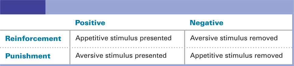
Figure 4.4 Positive and Negative Reinforcement and Punishment “Positive” means that something is presented, and “negative” means that something is taken away. Reinforcement means that the behavior is strengthened, and punishment means that the behavior is weakened. In positive reinforcement, an appetitive (pleasant) stimulus is presented, and in positive punishment, an aversive (unpleasant) stimulus is presented. In negative reinforcement, an aversive stimulus is removed, and in negative punishment, an appetitive stimulus is removed.

Similarly, in negative reinforcement and negative punishment, a stimulus is taken away. In negative reinforcement, an aversive stimulus is removed; in negative punishment, an appetitive stimulus is removed. An example of negative reinforcement would be taking Advil to get rid of a headache. The removal of the headache (an aversive stimulus) leads to continued Advil-taking behavior. An example of negative punishment would be taking away a teenager’s driving privileges after she breaks curfew. The removal of the driving privileges (an appetitive stimulus) leads to better adherence to the curfew in the future.

What type of operant conditioning is going on here? Be careful. Think about it from the perspectives of both the child and the parents. For the child, it’s positive reinforcement. The child is crying to get something pleasant (sleeping with the parents). For the parents, it’s negative reinforcement. They let the child sleep with them in order to remove something they find unpleasant, the crying.

©King Features Syndicate, Inc.

In all of these examples, however, we only know if a stimulus has served as a reinforcer or a punisher and led to reinforcement or punishment if the target behavior keeps occurring (reinforcement) or stops occurring (punishment). For example, the spanking would be punishment if the disobedient behavior stopped, and the praise reinforcement if the chores continued to be done. However, if the disobedient behavior continued, the spanking would have to be considered reinforcement; and if the chores did not continue to be done, the praise would have to be considered punishment. This is an important point. What serves as reinforcement or punishment is relative to each individual, in a particular context, and at a particular point in time. While it is certainly possible to say that certain stimuli usually serve as reinforcers or punishers, they do not inevitably do so. Think about money. For most people, $100 would serve as a reinforcer, but it might not for Bill Gates (of Microsoft), whose net worth is in the billions. Remember, whether the behavior is strengthened or weakened is the only thing that tells you whether the consequences were reinforcing or punishing, respectively.

Given the relative nature of reinforcement, it would be nice to have a way to determine whether a certain event would function as a reinforcer. The Premack principle provides us with a way to make this determination (Premack, 1959, 1965). According to David Premack, you should view reinforcers as behaviors rather than stimuli (e.g., eating food rather than food). This enables the conceptualization of reinforcement as a sequence of two behaviors—the behavior that is being reinforced followed by the behavior that is the reinforcer. But what is the principle? The principle is that the opportunity to perform a highly frequent behavior can reinforce performing a less frequent behavior. For example, children typically spend more time watching television than doing homework. Thus, watching television could be used as a reinforcer for doing homework. In sum, the Premack principle allows us to identify potential reinforcers by focusing on the relative probabilities of behaviors. To determine these probabilities, you observe how often the person or animal engages in various behaviors. The Premack principle has proved to be a very useful tool in applied work with clinical populations, situations in which normal reinforcers seem to have little effect, by enabling the identification of which behaviors will serve as reinforcers.

Primary and secondary reinforcers.

Behavioral psychologists make a distinction between primary and secondary reinforcers. A primary reinforcer is innately reinforcing, reinforcing since birth. Food and water are good examples of primary reinforcers. Note that “innately reinforcing” does not mean “always reinforcing.” For example, food would probably not serve as a reinforcer for someone who has just finished eating a five-course meal. Innately reinforcing only means that the reinforcing property of the stimulus does not have to be learned. In contrast, a secondary reinforcer is not innately reinforcing, but gains its reinforcing property through learning. Most reinforcers fall into this category. Examples of secondary reinforcers are money, good grades, and applause. Money would not be reinforcing to an infant, would it? Its reinforcing nature has to be learned through experience.

Behaviorists have employed secondary reinforcers in token economies in a variety of institutional settings, from schools to institutions for the mentally challenged (Allyon & Azrin, 1968). Physical objects, such as plastic or wooden tokens, are used as secondary reinforcers. Desired behaviors are reinforced with these tokens, which then can be exchanged for other reinforcers, such as treats or privileges. Thus, the tokens function like money in the institutional setting, creating a token economy. A token economy is an example of behavior modification—the application of conditioning principles, especially operant principles, to eliminate undesirable behavior and to teach more desirable behavior. Like token economies, other behavior modification techniques have been used successfully for many other tasks, from toilet training to teaching children who have autism (Kazdin, 2001).

Reinforcement without awareness.

According to behavioral psychologists, reinforcement should strengthen operant responding even when people are unaware of the contingency between their responding and the reinforcement. Evidence that this is the case comes from a clever experiment by Hefferline, Keenan, and Harford (1959). Participants were told that the purpose of the study was to examine the effects of stress on body tension and that muscular tension would be evaluated during randomly alternating periods of harsh noise and soothing music. Electrodes were attached to different areas of the participants’ bodies to measure muscular tension. The duration of the harsh noise, however, was not really random. Whenever a participant contracted a very small muscle in their left thumb, the noise was terminated. This muscular response was imperceptible and could only be detected by the electrode mounted at the muscle. Thus, the participants did not even realize when they contracted this muscle.

There was a dramatic increase in the contraction of this muscle over the course of the experimental session. The participants, however, did not realize this, and none had any idea that they were actually in control of the termination of the harsh noise. This study clearly showed that operant conditioning can occur without a person’s awareness. It demonstrated this using negative reinforcement (an increase in the probability of a response that leads to the removal of an aversive stimulus). The response rate of contracting the small muscle in the left thumb increased and the aversive harsh noise was removed when the response was made. Such conditioning plays a big role in the development of motor skills, such as learning to ride a bicycle or to play a musical instrument. Muscle movements below our conscious level of awareness but key to skill development are positively reinforced by our improvement in the skill.

Pessiglione et al. (2008) provide a more recent demonstration of operant conditioning without awareness for a decision-making task. In brief, participants learned to choose contextual cues predicting monetary reinforcement (winning money) relative to those predicting punishment (loss of money) without conscious perception of these cues. Thus, they learned cue-outcome associations without consciously perceiving the cues. The procedure involved visual masking. When a visual stimulus is masked, it is exposed briefly (for maybe 50 milliseconds) and followed immediately by another visual stimulus that completely overrides it, thereby masking (preventing conscious perception) of the first stimulus.

In this experiment, after being exposed to a masked contextual cue (an abstract novel symbol masked by a scrambled mixture of other cues) flashed briefly on a computer screen, a participant had to decide if he wanted to take the risky response or the safe response. The participant was told that the outcome of the risky response on each trial depended upon the cue hidden in the masked image. A cue could either lead to winning £1 (British currency), losing £1, or not winning or losing any money. If the participant took the safe response, it was a neutral outcome (no win or loss). Participants were also told that if they never took the risky response or always took it, their winnings would be nil and that because they could not consciously perceive the cues, they should follow their intuition in making their response decisions. All of the necessary precautions and assessments to ensure that participants did not perceive the masked cues were taken. Overall, participants won money in the task, indicating that the risky response was more frequently chosen following reinforcement predictive cues relative to punishment predictive cues.

In addition to this recent demonstration of operant conditioning without awareness, there have been several demonstrations of classical conditioning without awareness (Clark & Squire, 1998; Knight, Nguyen, & Bandetti, 2003; Morris, Öhman, & Dolan, 1998; Olsson & Phelps, 2004). Using delayed conditioning, Clark and Squire, for example, successfully conditioned the eyeblink response in both normal and amnesic participants who were not aware of the tone–air puff relationship. Participants watched a movie during the conditioning trials, and postconditioning testing indicated that they had no knowledge of the CS-UCS association.

General Learning Processes in Operant Conditioning

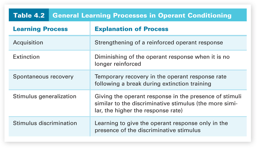
Now that we have a better understanding of how we learn through reinforcement and punishment, let’s consider the five general learning processes in operant conditioning that we discussed in the context of classical conditioning—acquisition, extinction, spontaneous recovery, generalization, and discrimination. Because some of the examples of these processes are concerned with operant conditioning of animals, it’s important to know how such animal research is conducted. It’s also important to learn how to read cumulative records because they are used to measure and depict operant responding in the general learning processes.

Craig Swanson perspicuity.com

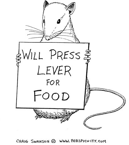
For control purposes, behavioral psychologists conduct much of their laboratory research on nonhuman animals. In conducting their experiments with animals, operant conditioning researchers use operant chambers, which resemble large plastic boxes. These chambers are far from simple boxes, though. Each chamber has a response device (such as a lever for rats to press or a key for pigeons to peck), a variety of stimulus sources (such as lamps behind the keys to allow varying colors to be presented on them), and food dispensers. Here, “key” refers to a piece of transparent plastic behind a hole in the chamber wall. The key or other response device is connected to a switch that records each time the animal responds. Computers record the animal’s behavior, control the delivery of food, and maintain other aspects of the chamber. Thus, the operant chamber is a very controlled environment for studying the impact of the animal’s behavior on its environment. Operant chambers are sometimes referred to as “Skinner boxes” because B. F. Skinner originally designed this type of chamber.

B. F. Skinner and one of his operant conditioning chambers, a “Skinner box.” When the rat presses the lever, an electrical relay system is activated and reinforcement (such as a food pellet) is delivered. In addition to a lever, operant chambers may contain other response mechanisms, such as a key for a pigeon to peck.

Nina Leen/Time-Life Pictures/Getty Images

What if the animal in the chamber does not make the response that the researcher wants to condition (for example, what if the pigeon doesn’t peck the key)? This does happen, but behavioral researchers can easily deal with this situation. They use what they call shaping; they train the animal to make the response they want by reinforcing successive approximations of the desired response. For example, consider the key-peck response for a pigeon. The researcher would watch the behavior of the pigeon and would begin the shaping by reinforcing the pigeon for going in the general area of the key. This would get the pigeon near the key. The researcher would then reinforce the pigeon any time its head was in the area of the key. The pigeon would keep its head near the key and would probably occasionally touch the key. Then the researcher would reinforce the pigeon for touching the key. As you can see, by reinforcing such successive approximations of the desired behavior, the animal can be shaped to make the desired response. This training by successive approximations is just as successful with humans and is also used to shape human operant responding.

Responding in an operant conditioning experiment is depicted in a cumulative record. A cumulative record is a record of the total number of responses over time. As such, it provides a visual depiction of the rate of responding. Figure 4.5 shows how to read a cumulative record. The slope of the record indicates the response rate. Remember that the record visually shows how the responses cumulate over time. If the animal is making a large number of responses per unit of time (a fast response rate), the slope of the record will be steep. The cumulative total is increasing quickly. When there is no responding (the cumulative total remains the same), the record is flat (no slope). As the slope of the record increases, the response rate gets faster. Now let’s see what cumulative records look like for some of the general learning processes.

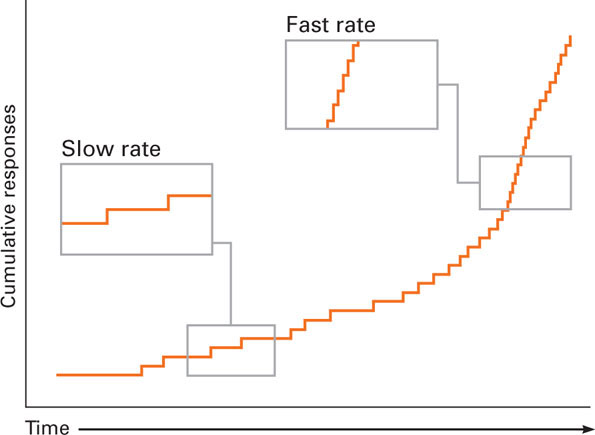Figure 4.5 How to Understand a Cumulative Record By measuring how responses cumulate over time, a cumulative record shows the rate of responding. When no responses occur, the record is flat (has no slope). As the number of responses increases per unit of time, the cumulative total rises more quickly. The response rate is reflected in the slope of the record. The faster the response rate, the steeper the slope of the record.

Acquisition, extinction, and spontaneous recovery.

The first general process, acquisition, refers to the strengthening of the reinforced operant response. What would this look like on the cumulative record? Figure 4.6(a) shows that the response rate increases over time. This looks very similar to the shape of the acquisition figure for classical conditioning (see Figure 4.2), but remember the cumulative record is reporting cumulative responding as a function of time, not the strength of the response. Thus, extinction, the diminishing of the operant response when it is no longer reinforced, will look different than it did for classical conditioning. Look at Figure 4.6(b). The decreasing slope of the record indicates that the response is being extinguished; there are fewer and fewer responses over time. The response rate is diminishing. When the record goes to flat, extinction has occurred. However, as in classical conditioning, there will be spontaneous recovery, the temporary recovery of the operant response following a break during extinction training. This would be indicated in the record by a brief period of increased responding following a break in extinction training. However, the record would go back to flat (no responding) as extinction training continued. This is shown in Figure 4.6(c).

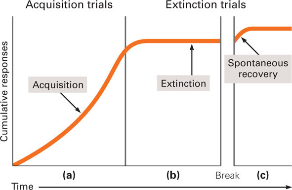Figure 4.6 Cumulative Record Illustrations of Acquisition, Extinction, and Spontaneous Recovery (a) This is an acquisition cumulative record; the responding rate increases as learning occurs so the cumulative record has a fairly steep slope reflecting this increase. (b) This is an extinction cumulative record; the responding rate has essentially fallen to zero. A flat cumulative record indicates extinction. (c) This is an example of spontaneous recovery—a burst of responding following a break in extinction training. As the extinction training continues, the record will return to flat (no responding).

Let’s think about acquisition, extinction, and spontaneous recovery with an example that is familiar to all of us—vending machines. We learn that by putting money into a certain vending machine, we can get a candy bar. We acquire the response of inserting money into this particular machine. One day, we put in money, but no candy comes out. This is the case the next few times we visit the machine. Soon, we stop putting our money in the machine. Our responding is being extinguished. However, after a few more days (a break), we go back and try again. This is comparable to spontaneous recovery. We hope the machine has been repaired, and we’ll get that candy bar. If so, our response rate will return to its previous level; if not, our response rate will continue along the extinction trail.

Discrimination and generalization.

Now let’s consider discrimination and generalization. To understand discrimination in operant conditioning, we need first to consider the discriminative stimulus—the stimulus that has to be present for the operant response to be reinforced or punished. The discriminative stimulus “sets the occasion” for the response to be reinforced or punished (rather than elicits the response as in classical conditioning). Here’s an example. Imagine a rat in an experimental operant chamber. When a light goes on and the rat presses the lever, food is delivered. When the light is not on, pressing the lever does not lead to food delivery. In brief, the rat learns the conditions under which pressing the lever will be reinforced with food. This is stimulus discrimination—learning to give the operant response (pressing the lever) only in the presence of the discriminative stimulus (the light). A high response rate in the presence of the discriminative stimulus (the light) and a near-zero rate in its absence would indicate that the discrimination was learned.

Now we can consider stimulus generalization, giving the operant response in the presence of stimuli similar to the discriminative stimulus. Let’s return to the example of the rat learning to press the lever in the presence of a light. Let’s make the light a shade of green and say that the rat learned to press the lever only in the presence of that particular shade of green light. What if the light were another shade of green, or a different color, such as yellow? Presenting similar stimuli (different-colored lights) following acquisition constitutes a test for generalization. The extent of responding to a generalization stimulus reflects the amount of generalization to that stimulus. As with classical conditioning (see Figure 4.3), there is a gradient of generalization in operant conditioning—as the generalization test stimulus becomes less similar to the discriminative stimulus, the response rate for the operant response goes down. A stimulus discrimination function similar to the one observed for classical conditioning would also be observed after additional discrimination training that involved teaching discrimination of the discriminative stimulus (the light) from other stimuli of the same class (lights of different colors).

Stimulus discrimination and generalization in operant conditioning are not confined to using simple visual and auditory stimuli such as colored lights and varying tones, even for animals other than humans. For example, Watanabe, Sakamoto, and Wakita (1995) showed that pigeons could successfully learn to discriminate paintings by Monet, an impressionist, and Picasso, a cubist; and that following this training, they could discriminate paintings by Monet and Picasso that had never been presented. Furthermore, the pigeons showed generalization from Monet’s paintings to paintings by other impressionists (Cezanne and Renoir) or from Picasso’s paintings to paintings by other cubists (Braque and Matisse). In addition, Porter and Neuringer (1984) have reported successful learning of musical discrimination between selections by Bach versus Stravinsky by pigeons followed by generalization to music by similar composers. Otsuka, Yanagi, and Watanabe (2009) similarly showed that even rats could learn this musical discrimination between selections by Bach versus those by Stravinsky. Thus, like humans, other animals can clearly learn to discriminate complex visual and auditory stimuli and then generalize their learning to similar stimuli.

All five of the general learning processes for operant conditioning are summarized in Table 4.2. If any of these processes are not clear to you, restudy the discussions of those processes in the text to solidify your understanding. Also make sure that you understand how these learning processes in operant conditioning differ from those in classical conditioning (summarized in Table 4.1.

Now that we understand the general processes involved in operant conditioning, we need to consider the question of how operant responding is maintained following acquisition. Will the responding be maintained if it is reinforced only part of the time? If so, what’s the best way to do this? Such questions require an understanding of what are called reinforcement schedules.

Partial-Reinforcement Schedules in Operant Conditioning

The reinforcement of every response is called a continuous schedule of reinforcement. But we aren’t reinforced for every response in everyday life. In real life, we experience partial schedules of reinforcement, in which a response is only reinforced part of the time. Partial-reinforcement schedules lead to the partial-reinforcement effect. Responses that are reinforced according to a partial schedule rather than a continuous schedule are more resistant to extinction. Incidentally, Skinner accidentally discovered the partial-reinforcement effect when he was short of food reinforcement for his experimental work and was forced to use partial reinforcement instead of continuous reinforcement (Skinner, 1956). To understand this effect, we first need to consider the four major aspects of partial-reinforcement schedules—ratio, interval, fixed, and variable.

Partial-reinforcement schedules can be based on either the number of responses made or on the amount of time that has elapsed. A ratio schedule is based on the number of responses made, and an interval schedule is based on the amount of time that has elapsed. In addition, the number of responses or the amount of elapsed time can be fixed or variable. In a fixed schedule, the number of responses required for a ratio schedule or the amount of time needed for an interval schedule is fixed. Similarly, for a variable schedule, the number of responses required for a ratio schedule and amount of time for an interval schedule varies on each trial. In summary, there are four types of partial schedules—fixed ratio, variable ratio, fixed interval, and variable interval. Let’s look first at ratio schedules.

Ratio schedules.

In a fixed-ratio schedule, a reinforcer is delivered after a fixed number of responses are made. The number of responses must be greater than one. (A fixed-ratio schedule that only required one response to get a reinforcer would be a continuous schedule of reinforcement). In a laboratory experiment, for example, a rat might have to press the lever 10 times (the fixed ratio) before the delivery of a reinforcer (usually food). To get another reinforcer, 10 more presses would be necessary, and so on. A good example from everyday life is piecework in a factory in which a worker has to make a certain number of items (say two wallets) before receiving any pay. The worker makes two wallets and then receives a certain amount of money. Then he or she must make two more to be paid that amount of money again. Just as the rat has to make responses (press the lever), the worker has to make responses (in this case, make actual products) to get reinforced.

John McPherson/Universal Press UClick

In a variable-ratio schedule, the number of responses it takes to obtain a reinforcer varies on each trial but averages to be a certain number across trials. The human, rat, or other animal never knows exactly how many responses will be necessary to get the next reinforcer. A rat might have to press a lever 10 times to get a reinforcer, then 21 times, then 6 times, and so on. The exact number of responses necessary to get a reinforcer varies. A good example in everyday life is the way a slot machine is programmed. The person playing the slot machine knows that it will eventually pay off but does not know how many responses (insertions of money into the slot machine) are necessary to get that payoff.

Ratio schedules lead to high rates of responding because the number of responses determines reinforcement; the more they respond, the more they are reinforced. Cumulative records for the two ratio schedules are given in Figure 4.7. The slopes for the two ratio schedules are steep, which indicates a high rate of responding. Look closely after each reinforcement presentation (indicated by a tick mark), and you will see very brief pauses after reinforcement, especially for the fixed-ratio record. These pauses indicate that the animal took a short break from responding following the reinforcement. These pauses occur more often for the fixed-ratio schedule because the number of responses that must be made to get another reinforcer is known. Thus, the animal or human can rest before starting to respond again. These pauses get longer as the fixed number of responses gets larger.

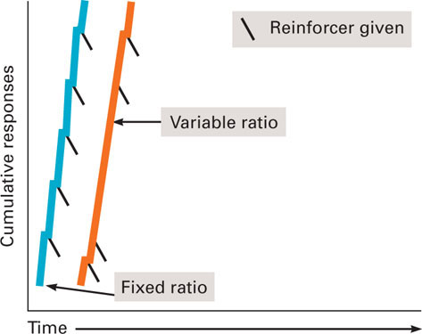Figure 4.7 Cumulative Records for Fixed-Ratio and Variable-Ratio Schedules of Partial Reinforcement Both ratio schedules lead to high rates of responding as indicated by the steep slopes of the two cumulative records. Each tick mark indicates when a reinforcer was delivered. As you can see, the tick marks appear regularly in the record for the fixed-ratio schedule, but irregularly in the record for the variable-ratio schedule. A fixed-ratio schedule leads to short pauses after reinforcement, but these pauses don’t occur as often for a variable-ratio schedule.

Interval schedules.

Now let’s consider interval schedules. Do you think the cumulative records for the two interval schedules will have steep slopes like the two ratio schedules? Will there be any flat sections in the record indicating no responding? Let’s see. In a fixed-interval schedule, a reinforcer is delivered following the first response after a set interval of time has elapsed. Please note that the reinforcement does not automatically appear after the fixed interval of time has elapsed; the reinforcement merely becomes obtainable after the fixed interval. A response must be made in order to get the reinforcement. Let’s consider an example. We could fix the time interval at one minute for our example of a rat pressing a lever in an operant chamber. This means that a food pellet would be delivered following the first lever press after one minute had elapsed. After another minute elapsed following the response and another lever press was made, another reinforcer would be delivered. This pattern would continue—one minute elapses, a response is made, a reinforcer is given. Before predicting what the cumulative record for this type of schedule should look like, let’s think about a fixed-interval schedule example with students.

In most of your classes, you are given periodic scheduled exams (for example, an exam every four weeks). To understand how such periodic exams represent a fixed-interval schedule, think of studying as the targeted response, and an acceptable grade on the exam as the reinforcer. Think about how much you would study during each of the four-week intervals before each test. Think about the average study behavior across students in the class for each day during that four-week interval. There probably wouldn’t be much studying during the first week or two, and the amount of study would increase dramatically (cramming) right before each exam. Think about what the cumulative record for this sort of responding would look like. There would be long periods with little responding (essentially flat sections) right after each exam, and then there would be a dramatic burst of responding (a steep slope) right before each exam. Now look at the record for the fixed-interval schedule in Figure 4.8. It looks just like this. This is also what the record would look like for a rat pressing a lever on this type of schedule for a food reinforcer.

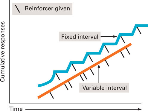Figure 4.8 Cumulative Records for Fixed-Interval and Variable-Interval Schedules of Partial Reinforcement As in Figure 4.7, the tick marks indicate when reinforcers were delivered for each of the two schedules. The flat sections following reinforcements for the fixed-interval schedule indicate periods when little or no responding occurred. Such pauses do not occur for a variable-interval schedule. A variable-interval schedule leads to steady responding.

Now imagine that you are the teacher of a class in which students had this pattern of study behavior. How could you change the students’ study behavior to be more regular? The answer is to use a variable-interval schedule in which a reinforcer is delivered following a response after a different time interval on each trial (in our example, each exam), but the time intervals across trials average to be a set time. This would translate in our example to unscheduled surprise exams. Think about how students’ study behavior would have to change to do well on the exams with this new schedule. Students would have to study more regularly because a test could be given at any time. Their studying would be steadier over each interval. They wouldn’t have long periods of little or no studying. Now look at the cumulative record for the variable-interval schedule in Figure 4.8. The flat sections appearing in the fixed-interval schedule are gone. The slope of the record indicates a steady rate of responding (studying). Why? The answer is simple—the length of the interval varies across trials (between exams in the example). It might be very brief or very long. The students don’t know. This is why the responding (studying) becomes steady.

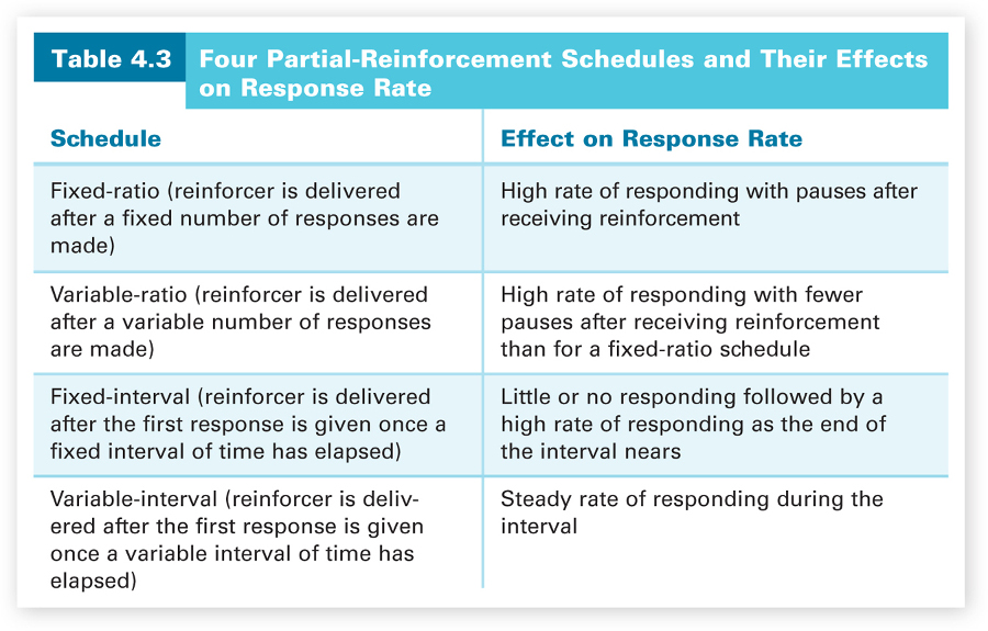
The four types of partial-reinforcement schedules and their respective effects on response rate are summarized in Table 4.3. As you review the information in this table for each type of schedule, also review the cumulative record for the schedule in either Figure 4.7 or Figure 4.8 to see visually the impact of that type of schedule upon responding.

Let’s compare the cumulative records for the four types of partial-reinforcement schedules given in Figure 4.7 and Figure 4.8. What conclusions can we draw? First, ratio schedules lead to higher rates of responding than interval schedules. Their slopes are much steeper. This is because ratio schedules depend on responding, and interval schedules depend on time elapsing. Second, variable schedules lead to fewer breaks (periods during which no responding occurs) after reinforcements than fixed schedules. This is because with variable schedules it is not known how many responses will have to be made or how much time will have to elapse before the next reinforcement.

Now let’s think about partial-reinforcement schedules in terms of a general learning process—extinction. Remember the partial-reinforcement effect that we described at the beginning of this section—partial schedules of reinforcement are more resistant to extinction than are continuous schedules. This means that responding will not be extinguished as quickly after using one of the partial schedules as it would be with a continuous schedule. Obviously, it is easier to extinguish the response if the reinforcement had been given continuously for every response in the past. If a response is made and doesn’t get reinforced, the responder knows immediately something is wrong because they have always been reinforced after each response. With partial schedules, if a response is made and doesn’t get reinforced, the responder doesn’t know that anything is wrong because they have not been reinforced for every response. Thus, it will take longer before extinction occurs for the partial schedules because it will take longer to realize that something is wrong.

Do you think there are any differences in this resistance to extinction between the various partial schedules of reinforcement? Think about the fixed schedules versus the variable schedules. Wouldn’t it be much more difficult to realize that something is wrong on a variable schedule? On a fixed schedule, it would be easy to notice that the reinforcement didn’t appear following the fixed number of responses or fixed time interval. On a variable schedule, however, the disappearance of reinforcement would be very difficult to detect because it’s not known how many responses will have to be made or how much time has to elapse. Think about the example of a variable-ratio schedule with the rat pressing a lever. Because there is no fixed number of responses that have to be made, the rat wouldn’t realize that its responding was being extinguished. It could be that the number of lever presses necessary to get the next reinforcement is very large. Because of such uncertainty, the variable schedules are much more resistant to extinction than the fixed schedules.

Motivation, Behavior, and Reinforcement

We have just learned about how reinforcement works and that partial-reinforcement schedules are powerful. But what initiates our behavior and guides it toward obtaining reinforcement? The answer is motivation, the set of internal and external factors that energize our behavior and direct it toward goals. Its origin is the Latin word movere, meaning to set in motion. Motivation moves us toward reinforcement by initiating and guiding our goal-directed behavior. There are several explanations of how motivation works. We will first consider a few general theories of motivated behavior and then a distinction between two types of motivation and reinforcement, extrinsic versus intrinsic.

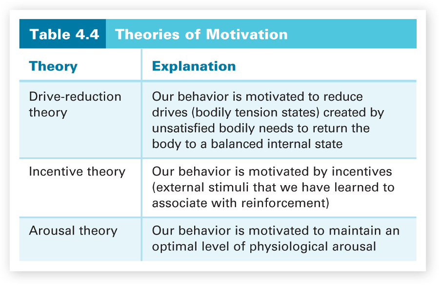
Theories of motivation.

One explanation of motivation, drive-reduction theory, proposes that first, a bodily need (such as hunger) creates a state of bodily tension called a drive; then, motivated behavior (seeking food) works to reduce this drive by obtaining reinforcement (food) to eliminate this need and return the body to a balanced internal state. Drives are disruptions of this balanced bodily state. We are “pushed” into action by these unpleasant drive states. They motivate our behavior to reduce the drive. Drive-reduction theory does a good job of explaining some of our motivated behaviors, especially those concerned with biological needs, such as hunger and thirst; but it cannot explain all motivated behavior. Our behaviors are clearly motivated by factors other than drive reduction. Even eating and drinking aren’t always cases of drive-reduction motivation. What if you accidentally run into someone that you really want to date and she/he asks you to lunch, but you had eaten a full lunch 15 minutes earlier? You would probably eat another lunch, wouldn’t you? We eat for reasons other than hunger. Similarly, I’m sure that you often drink beverages without being truly thirsty. And is it really a “thirst” for knowledge that motivates your study behavior? A complementary theory, the incentive theory of motivation, has been proposed to account for such behavior.

In contrast to being “pushed” into action by internal drive states, the incentive theory of motivation proposes that we are “pulled” into action by incentives, external environmental stimuli that do not involve drive reduction. The source of the motivation, according to incentive theory, is outside the person. Money is an incentive for almost all of us. Good grades and esteem are incentives that likely motivate much of your behavior to study and work hard. Incentive theory is much like operant conditioning. Your behavior is directed toward obtaining reinforcement.

Another explanation of motivation, arousal theory, extends the importance of a balanced internal environment in drive-reduction theory to include our level of physiological arousal and its regulation. According to arousal theory, our behavior is motivated to maintain an optimal level of arousal, which varies within individuals (Zuckerman, 1979). When below the optimal level, our behavior is motivated to raise our arousal to that level. We seek stimulation. We might, for example, go see an action movie. If overaroused, then our behavior is motivated to lower the arousal level. We seek relaxation, so we might take a nap or a quiet walk. So in arousal theory, motivation does not always reduce arousal as in drive-reduction theory, but rather regulates the amount of arousal (not too much, not too little).

In addition, arousal theory argues that our level of arousal affects our performance level, with a certain level being optimal. Usually referred to as the Yerkes-Dodson law because Robert Yerkes and James Dodson (1908) originally proposed it, this relationship between level of arousal and performance quality is rather simple. Shown in Figure 4.9, it is an inverted U–shaped relationship. Increased arousal will aid performance to a point (the optimal amount of arousal), after which further arousal impairs performance. Think about exams. You need to be aroused to do well on them; but if you are too aroused, your performance will be negatively affected.

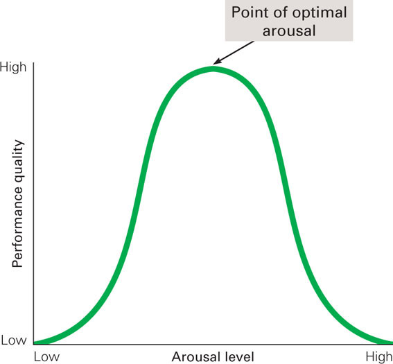Figure 4.9 The Yerkes-Dodson Law The Yerkes-Dodson law is very straightforward. As arousal increases, the quality of performance increases—up to the point of optimal arousal. Further increases in arousal are detrimental to performance.

To solidify your understanding of these three theories of motivation, they are summarized in Table 4.4.

Extrinsic motivation versus intrinsic motivation.

Motivation researchers make a distinction between extrinsic motivation, the desire to perform behavior to obtain an external reinforcer or to avoid an external aversive stimulus, and intrinsic motivation, the desire to perform a behavior for its own sake. In cases of extrinsic motivation, reinforcement is not obtained from the behavior, but is a result of the behavior. In intrinsic motivation, the reinforcement is provided by the activity itself. Think about what you are doing right now. What is your motivation for studying this material? Like most students, you want to do well in your psychology class. You are studying for an external reinforcer (a good grade in the class), so your behavior is extrinsically motivated. If you enjoy reading about psychology and studying it for its own sake and not to earn a grade (and I hope that you do), then your studying would be intrinsically motivated. It is not an either-or situation. Both types of motivation are probably involved in your study behavior, but the contribution of each type varies greatly for each student.

The reinforcers in cases of extrinsic motivation—such as food, money, and awards—are called extrinsic reinforcers. They do not originate within the task itself, but come from an external source. In the case of intrinsic motivation, the enjoyment of the behavior and the sense of accomplishment from it are labeled intrinsic reinforcers. Paradoxically, researchers have found that extrinsic reinforcement will sometimes undermine intrinsically motivated behavior (Deci, Koestner, & Ryan, 1999; Lepper & Henderlong, 2000; Tang & Hall, 1995). This is referred to as the overjustification effect, a decrease in an intrinsically motivated behavior after the behavior is extrinsically reinforced and then the reinforcement is discontinued.

The overjustification effect has been demonstrated for people of all ages, but let’s consider an example from a study with nursery-school children (Lepper, Greene, & Nisbett, 1973). The children liked drawing with felt-tip pens and did so during play periods (they were intrinsically motivated to engage in such drawing). Once this was established, some of the children were given extrinsic reinforcement—“Good Player” awards—for their drawing, under the guise that someone was coming to look at the children’s drawings. Other children were not given this extrinsic reinforcement for drawing. A week later, when no certificates were being offered for the felt-tip drawings, the children who had not been extrinsically reinforced continued to draw with the felt-tip pens, but those who had been reinforced spent much less time drawing, illustrating the overjustification effect. What leads to this effect?

In our example, extrinsic reinforcement (the awards for the children) provides unnecessary justification for engaging in the intrinsically motivated behavior (drawing with the felt-tip pens). A person’s intrinsic enjoyment of an activity provides sufficient justification for their behavior. With the addition of the extrinsic reinforcement, the person may perceive the task as overjustified and then attempt to understand their true motivation (extrinsic versus intrinsic) for engaging in the activity. It is this cognitive analysis of motivation that leads to the decrease in engaging in the activity. In this cognitive analysis, the person overemphasizes the importance of the extrinsic motivation to their behavior. For example, the person may perceive the extrinsic reinforcement as an attempt at controlling their behavior, which may lead them to stop engaging in the activity to maintain their sense of choice. A person might also think that the reinforcement makes the activity more like work (something one does for extrinsic reinforcement) than play (something one does for its own sake), lessening their enjoyment of the activity and leading them to cease engaging in it.

The overjustification effect indicates that a person’s cognitive processing influences their behavior and that such processing may lessen the effectiveness of extrinsic reinforcers. Don’t worry, though, about the overjustification effect influencing your study habits (assuming that you enjoy studying). Research has shown that performance-contingent extrinsic reinforcers (such as your grades, which are contingent upon your performance) are not likely to undermine studying (Eisenberger & Cameron, 1996; Tang & Hall, 1995). This means that the extrinsic reinforcement is not likely to impact intrinsic motivation if the extrinsic reinforcement is dependent upon doing something well versus just doing it.

The overjustification effect imposes a limitation on operant conditioning and its effectiveness in applied settings. It tells us that we need to be careful in our use of extrinsic motivation so that we do not undermine intrinsic motivation. It also tells us that we must consider the possible cognitive consequences of using extrinsic reinforcement. In the next section, we continue this limitation theme by first considering some biological constraints on learning and then some cognitive research that shows that reinforcement is not always necessary for learning.