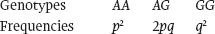
21.3 EVOLUTION AND THE HARDY–WEINBERG EQUILIBRIUM

Determining allele frequencies gives us information about genetic variation. Following that variation over time is key to understanding the genetic basis of evolution.

21.3.1 Evolution is a change in allele or genotype frequency over time.

At the genetic level, evolution is simply a change in the frequency of an allele or a genotype from one generation to the next. For example, if there are 200 copies of an allele that causes blue eye color in a population in generation 1 and there are 300 copies of that allele in a population of the same size in generation 2, evolution has occurred. In principle, evolution may occur without allele frequencies changing. For instance, even if, in our fruit fly example, the A/G allele frequencies stay the same from one generation to the next, the frequencies of the different genotypes (that is, of AA, AG, and GG) may change. This would be evolution without allele frequency change.

Evolution is therefore a change in the genetic makeup of a population over time. Note an important and often misunderstood aspect of this definition: populations evolve, not individuals. Note, too, that this definition does not specify a mechanism for this change. As we will see, many mechanisms can cause allele or genotype frequencies to change. Regardless of which mechanisms are involved, any change in allele frequencies, genotype frequencies, or both constitutes evolution.

21.3.2 The Hardy–Weinberg equilibrium describes situations in which allele and genotype frequencies do not change.

Allele and genotype frequencies change over time only if specific mechanisms act on the population. This principle was demonstrated independently in 1908 by the English mathematician G. H. Hardy and the German physician Wilhelm Weinberg, and has become known as the Hardy–Weinberg equilibrium. In essence, the Hardy–Weinberg equilibrium is the situation in which evolution does not occur.

The Hardy–Weinberg equilibrium specifies the relationship between allele frequencies and genotype frequencies when a number of key conditions are met. When these conditions are met—and the Hardy–Weinberg equilibrium holds—we can conclude that evolutionary mechanisms are not acting on the gene in the population we are studying. In many ways, then, the Hardy–Weinberg equilibrium is most interesting when we find instances in which allele or genotype frequencies depart from expectations. This finding implies that one or more of the conditions are not met and that evolutionary mechanisms are at work.

These are the required conditions for the Hardy–Weinberg equilibrium:

1. There can be no differences in the survival and reproductive success of individuals. Given two alleles, A and a, imagine an extreme case in which a, a recessive mutation, is lethal. All aa individuals die. Therefore, in every generation, there is a selective elimination of a alleles, meaning that the frequency of a will gradually decline (and the frequency of A correspondingly increase) over the generations. As we discuss below, we call this differential success of alleles selection.
2. Populations must not be added to or subtracted from by migration. Imagine a second population adjacent to the one we used in the preceding example in which all the alleles are A and all individuals have the genotype AA. Recall that when a population has only one allele of a particular gene, it is fixed for that allele. Now imagine that there is a sudden influx of individuals from the first population into the second. The frequency of A in the second population will change in proportion to the number of immigrants.
3. There can be no mutation. If A alleles mutate into a alleles, and vice versa, then again we will see changes in the allele frequencies over the generations. In general, because mutation is so rare, it is not a serious consideration on the timescales studied by population geneticists. However, as we have seen, mutation is the ultimate source of genetic variation, so it is a key input on which other evolutionary mechanisms act.
4. The population must be sufficiently large to prevent sampling errors. Chance events are more likely in small samples than in large ones. Campus-wide, a college’s sex ratio may be close to 50:50, but in a small class of 8 individuals it is not improbable that we would have 6 women and 2 men (a 75:25 ratio). Sample size, in the form of population size, also affects the Hardy–Weinberg equilibrium such that it technically holds only for infinitely large populations. A change in the frequency of an allele due to the random effects of small population size is called genetic drift.
5. Individuals must mate at random. For the Hardy–Weinberg equilibrium to hold, mate choice must be made without regard to genotype. For example, an AA homozygote when offered a choice of mate from among AA, Aa, or aa individuals should choose at random. In contrast, non-random mating occurs when individuals do not mate randomly. For example, AA homozygotes might preferentially mate with other AA homozygotes. Non-random mating affects genotype frequencies from generation to generation, but does not affect allele frequencies.

21.3.3 The Hardy–Weinberg equilibrium translates allele frequencies into genotype frequencies.

Now that we have established the conditions required for a population to be in Hardy–Weinberg equilibrium, let us explore the idea in detail. In the example we looked at earlier, we know the frequency of the two alleles, one with A and the other with G in the Adh gene in Drosophila. What are the genotype frequencies? That is, how many AA homozygotes, AG heterozygotes, and GG homozygotes do we see? The Hardy–Weinberg equilibrium predicts genotype frequencies from allele frequencies.

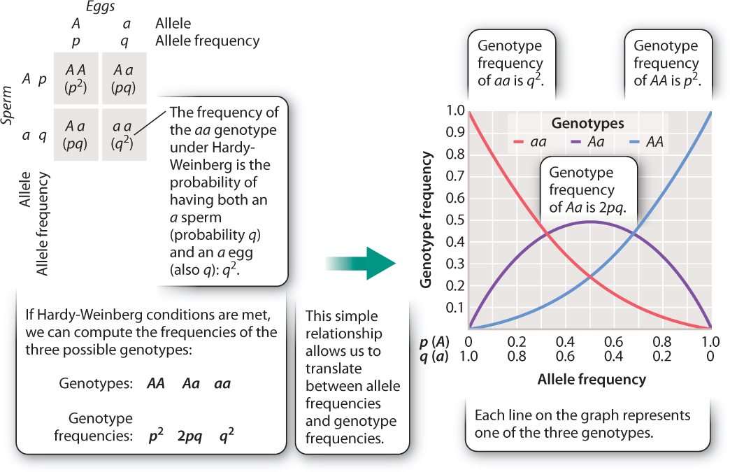
The logic is simple. Random mating is the equivalent of putting all the population’s gametes into a single pot and drawing out pairs of them at random to form a zygote. We therefore put in our 70 A alleles and 30 G alleles and pick pairs at random. What is the probability of picking an AA homozygote (that is, what is the probability of picking an A allele followed by another A allele)? The probability of picking an A allele is its frequency in the population, so the probability of picking the first A is 0.7. What is the probability of picking the second A? Also 0.7. What then is the probability of picking an A followed by another A? It is the product of the two probabilities: 0.7 × 0.7 = 0.49. Thus, the frequency of an AA genotype is 0.49. We take an identical approach to determine the genotype frequency for the GG genotype: Its frequency is 0.3 × 0.3, or 0.09.

What about the frequency of the heterozygote, AG? This is the probability of drawing G followed by A, or A followed by G. There are thus two separate ways in which we can generate the heterozygote. Its frequency is therefore (0.7 × 0.3) + (0.3 × 0.7) = 0.42.

We can generalize these calculations algebraically by substituting letters for the numbers we have computed to derive the Hardy–Weinberg equilibrium. If the allele frequency of one allele, A, is p, and the other, G, is q, then

p + q = 1 (because there are no other alleles at this site).

Not only do these relationships predict genotype frequency from allele frequencies, but they work in reverse, too. Fig. 21.5 shows how Hardy–Weinberg values are calculated from allele frequencies and, in the graph on the right, how allele and genotype frequencies are related. Note that we can use the graph to determine both allele frequencies for a given genotype frequency (to take a simple case, a 0.5 frequency of heterozygotes, Aa, implies that both p and q are 0.5) and genotype frequencies for a specified allele frequency.

Figure 21.5: Hardy-Weinberg Relation. The Hardy-Weinberg relation predicts genotype frequencies from allele frequencies, and vice versa.

We can do this mathematically as well. Knowing the genotype frequency of AA, for example, permits us to calculate allele frequencies: if, as in our Adh example, p² is 0.49 (that is, 49% of the population has genotype AA), then p, the allele frequency of A, is Because p + q = 1, then q, the allele frequency of a, is 1 – 0.7 = 0.3.

Note that these relationships hold only if the Hardy–Weinberg conditions are met. If not, then allele frequencies can only be deduced by tallying alleles from genotype frequencies as described earlier in section 21.2.

21.3.4 The Hardy–Weinberg equilibrium is the starting point for population genetic analysis.

Recall our definition of evolution: a change in allele or genotype frequency from one generation to the next. Given this definition, it might seem odd to be discussing factors necessary for allele frequencies to stay the same. The Hardy–Weinberg equilibrium not only provides a means of converting between allele and genotype frequencies, but, critically, it also serves as an indicator that something interesting is happening in a population when it is not upheld.

If we find a population whose allele or genotype frequencies are not in Hardy–Weinberg equilibrium, we can infer that evolution has occurred. We can then consider, for the gene under study, whether the population is subject to selection, migration, mutation (unlikely because of its rarity), genetic drift, or non-random mating. These are the primary mechanisms of evolution. The Hardy–Weinberg equilibrium gives us a baseline from which to explore the evolutionary processes affecting populations. We will start by considering one of the most important evolutionary mechanisms: natural selection.