46.1 POPULATIONS AND THEIR PROPERTIES

When the first United States census was completed in 1790, the British scholar Thomas Malthus supposed that the remarkable recent growth of the American population, which had doubled in the previous 25 years, was a consequence of ample food supply and the active encouragement of marriages, neither of which characterized Europe at the time. In his 1798 volume An Essay on the Principle of Population, Malthus argued that a similar periodic doubling of population in the British Isles, on the other hand, would outstrip the more slowly increasing food supply in 50 years and lead to starvation. That is, increasing the number of births per year would eventually result in an increased number of deaths because the amount of food the land could produce was limited. This view of the human condition would influence the thinking of Charles Darwin, who as a young, inquisitive student read the most exciting works of the day. Darwin realized that the tension between population growth and resource limitation applies to all species, leading to a struggle for existence that results in adaptations that enhance survival (Chapter 21).

In Chapter 21, we introduced the concept of population as a fundamental unit of evolution—it is populations, and not individuals, that evolve. Here, we return to populations, this time as equally fundamental units of ecology. A population consists of all the individuals of a given species that live and reproduce in a particular place. Natural selection enables populations to adapt to the physical and biological components of their environment. It is the traits evolved under natural selection that determine whether a population will succeed or fail under a given set of physical and biological conditions—whether it will grow and expand its range or shrink, perhaps disappearing entirely from a local environment.

What controls changes in population size? We first look at what happens when there are more births than deaths. We then examine what happens when resources such as food start to run out. We consider how individuals of different ages contribute to population growth, and finally, in the next chapter, we introduce interactions with other species and see how they shape the growth of a population. All these factors directly influence the flow of energy and materials through producers and consumers and, ultimately, the flow of genes through a population.

46.1.1 Three key features of a population are its size, range, and density.

Figure 46.1: (a) Size, (b) range, and (c) density of a population. The places where populations occur can be mapped, and the numbers of individuals within those populations can be estimated. This information helps us understand what factors limit population distributions.

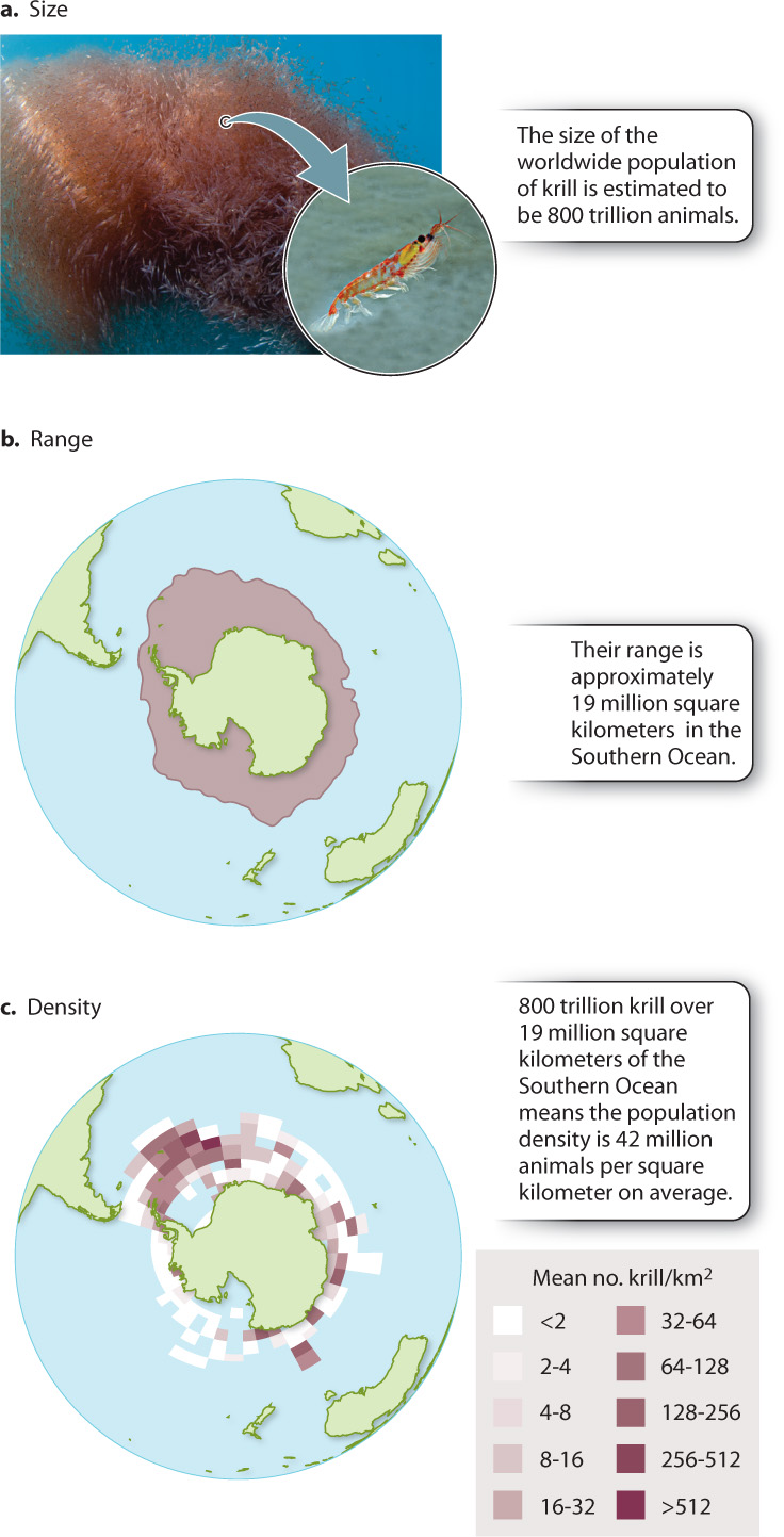
Populations are defined by three key features: size, range, and density (Fig. 46.1). Population size is simply the number of individuals of all ages alive at a particular time in a particular place. For example, the population of krill in the cold waters around Antarctica is estimated to be 800 trillion, making them by mass the most abundant animals on Earth (Fig. 46.1a).

The size of a population may increase, decrease, or stay the same over time, and trends in population size are a key focus of ecological research and its application to conservation biology. A decrease in size through time, for example, might signal declining health in a local population—a matter of practical concern when the population in question is a commercially harvested fish or an endangered species. In the 1990s, catastrophic declines in cod populations led to a ban on commercial cod fishing on the Grand Banks of Newfoundland. The decline affected both cod and cod fishers, and it also led to changes in Grand Banks ecosystems—crab and lobster populations have increased as predation pressure by cod has declined.

A second key feature of a population is its geographic range: how widely a population is spread out. Fig. 46.1b, for example, shows that the krill population ranges through an area of 19 million square kilometers around Antarctica. The geographic range of any species determines how much variation in climate a population can tolerate and how many other species the population encounters. The geographic range of a plant population, for example, influences how many kinds of insect eat it, and the size of the range of an insect determines how many kinds of plant it encounters.

Taken together, population size and range contribute to a third key attribute of a population, its density: how crowded or dispersed the individuals are that make up the population. Population density is defined as a population’s size divided by its range. For krill, 800 trillion animals are spread over 19 million square kilometers—a density of 42 million animals per square kilometer (Fig. 46.1c). As we will see, population density can affect population size.

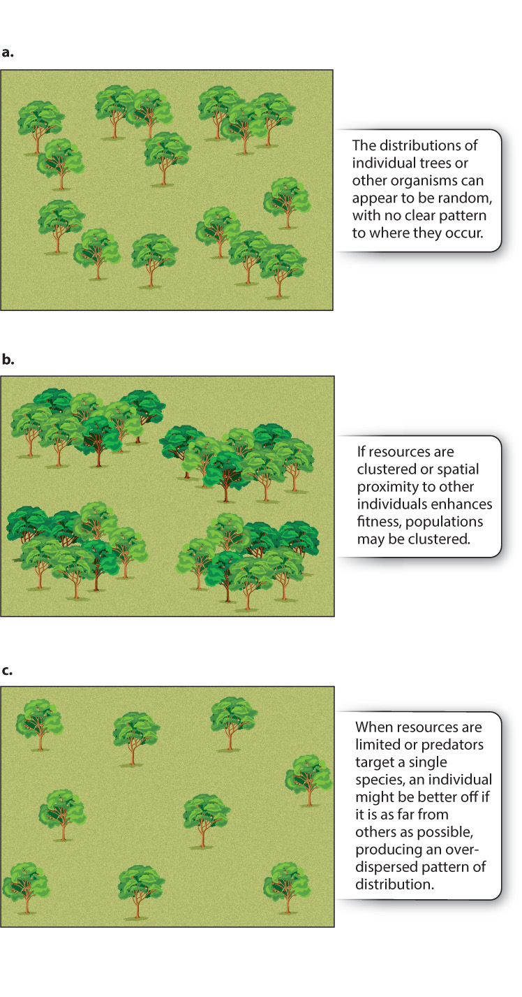
This way of characterizing population density, as average density across the range of a species, is often useful, but it can be misleading if organisms occur unevenly within their range. In nature, the individuals within a population may be distributed randomly—that is, a new individual has an equal chance of occupying any position within the range, and the location of one individual has no influence on where the next will occur (Fig. 46.2a). Sometimes, however, resources are distributed patchily within the range, or the chances of a new individual’s surviving are enhanced by the presence of other individuals. In these circumstances, the population may be clumped, with individuals clustered together (Fig. 46.2b). In some cases, one individual of a population might prevent another from settling nearby, for example if all individuals depend on the same set of resources. Or, predators, having located one prey individual, may search for other members of the same species nearby. Ecologists call such populations overdispersed, meaning that they are distributed more nearly uniformly than would be predicted by chance (Fig. 46.2c). Also, habitats suitable for growth may themselves occur in isolated patches. We discuss the implications of habitat patchiness in greater detail later in the chapter.

Figure 46.2: Distribution of individuals within populations. A population may be (a) randomly distributed, (b) clumped, or (c) overdispersed.

46.1.2 Population size can increase or decrease over time.

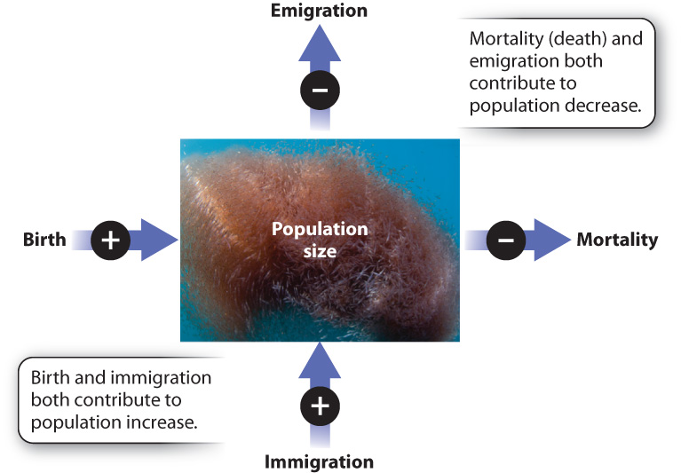
Many factors affect population size. An obvious process that contributes to population increase is birth. Another is immigration: Individuals may arrive in a population from elsewhere. In contrast, mortality (death) and emigration, the departure of individuals from a population, both act to decrease population size (Fig. 46.3).

Figure 46.3: Factors affecting the size of a population: birth, mortality, immigration, and emigration.

Population size changes continually as individuals are born or immigrate into the population, and as they die or emigrate away from a population. We can describe the changes in a population’s size mathematically, defining population size as N and the change in population time over a given time interval as ∆N, where the Greek letter ∆ (delta) means “change in.” ∆N is the number of individuals at a given time (time 2) minus the number of individuals at an earlier time (time 1), which is symbolized as N₂ − N₁. As the processes leading to a change in population size through time include births (B), deaths (D), immigration (I), and emigration (E), we can quantify ∆N as:

∆N = N₂ − N₁ = (B − D) 1 (I − E)

Commonly, ecologists want to know not just whether population size is increasing or decreasing, but also the rate at which population size is changing—that is, the change in population size (∆N) in a given period of time (∆t), or ∆N/∆t. Let’s say a population starts with 80 individuals and after 2 years has grown to 120 individuals. The population, then, has gained 40 individuals in 2 years, for a rate of 40/2 = 20 individuals per year.

The importance we place on such a number strongly depends on the actual population size. An increase of 20 individuals in a year is a big deal if the starting population had 80 individuals, but it is small if the starting population numbered 10,000. Usually, therefore, we are most interested in the proportional increase or decrease over time, especially the growth rate per individual, or the per capita growth rate (capita in Latin means “head”). The per capita growth rate is commonly symbolized by r and is calculated as the change in population size per unit of time divided by the number of individuals at the start (time 1):

r = (∆N/∆t)/N₁

In our example above, r equals 20 individuals per year divided by 80 individuals, for a per capita growth rate of 0.25 per year.

It is important to realize that while rates are important in ecology, the data we usually have in hand actually consist of the numbers of individuals that we have counted, and we often do not know exactly how large a natural population really is and so must rely on estimates. We consider how we make such population size estimates later in this chapter, but for the rest of this discussion we focus on the per capita increase (or decrease) in a population over time and assume we know the population sizes for species of interest.

In the example discussed in the preceding paragraphs, an initial population of 80 individuals increased by 20 per year, numbering 120 after 2 years, for a per capita rate of increase of 0.25 per year. Should this per capita rate of increase continue, how large will the population be after 10 years? We can answer this question using the following formula:

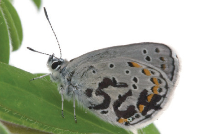
N_t = N₁(1 + r)^t

The population size after 10 years (N_t, where t = 10) will equal the initial population size (N₁ = 80) times 1 plus the per capita growth rate (0.25) raised to the power t (10 years). Solving the equation for our example shows that in 10 years the population size would be 745. After 15 years, the population would swell to 2273.

Figure 46.4: Exponential growth. When per capita growth rate, r, is constant, the curve shows ever-larger changes in population size over time.

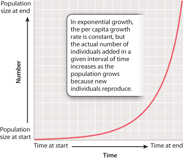
This example illustrates exponential growth, the pattern of population increase that results when r is constant through time. A prominent feature of exponential growth is that the number of individuals added to the population in any time interval is proportional to the size of the population at the start of the interval. That is, while the per capita growth rate remains constant, the actual number of individuals added per time unit increases as the population grows. This is because the new individuals added also reproduce themselves, so through time more and more individuals contribute to the growing population. Fig. 46.4 shows the characteristic shape of an exponential growth curve.

A second example brings home the remarkable consequences of exponential growth. A chessboard has 8 rows of 8 squares each, a total of 64 squares. Suppose we place a grain of wheat on the first square of the chessboard, two on the second square, four on the third, and keep doubling the number at each successive square. By the time we reach the 64th square, the total number of grains on the board is 18,446,744,073,709,551,615, more than 80 times what the Earth could produce in a year if wheat were planted on every square inch of farmland, and about a million times the number of stars in the Milky Way galaxy.

The per capita growth rate, r, is commonly called the intrinsic growth rate of a population, the maximum rate of growth when no environmental factors limit population increase. Intrinsic rates of growth in mammals range from 82% per year in muskrats to 50% in snowshoe hares and 10% in moose. Malthus recognized that exponential growth cannot continue for long in nature because the number of individuals will eventually outstrip the resources available to support the population. Darwin, in turn, recognized that when the number of young produced at birth exceeds the number of adults that can be supported by available resources, individuals within the population will compete to obtain the resources needed for growth and reproduction. This intraspecific (within-species) competition results in natural selection (Chapter 21), linking the ecological and evolutionary aspects of populations. Individuals from different species can also compete for resources. Such interspecific (between-species) competition can result in an increase or decrease in population size. We focus for the most part on intraspecific competition in this chapter, reserving a detailed discussion of the effects of interspecific competition until Chapter 47.

46.1.3 Carrying capacity is the maximum number of individuals a habitat can support.

As a population grows, crowding commonly results in a decrease in the availability or quality of resources required for continuing growth. As a consequence, growth rate declines. On Hispaniola, for example, Lime Swallowtails have probably reached the limit of available citrus groves. Individual females have to search longer to find suitable plants that do not have eggs already laid by other females. With that delay, and the pressure of eggs that are continuing to mature inside their bodies, females may end up laying too many eggs in one place or on poor-quality food, so there is not enough food for all larvae to survive. All of these factors lead to fewer births than occurred immediately after the Lime Swallowtails first arrived in Hispaniola, when resources were not limiting.

For many organisms, crowding affects the death rate as well as the birth rate. For example, as the fish population of a pond increases, there is less food available for each individual, and oxygen may be used up by microbes that proliferate because of nutrients in the fish waste.

In other words, birth and death rates are themselves affected by population density, which we defined earlier as the number of individuals per unit of area or (for aquatic species) volume of habitat. Increasing density is not always detrimental to a population. For example, eggs of a salmon or sturgeon are more likely to be fertilized in rivers or streams swarming with their species than when there are few reproducing adults. Generally, however, at some point increasing population density causes the environment to deteriorate because of a scarcity of resources. When the density of a growing population reaches this point, the rate of growth slows and eventually levels off as the death rate increases to equal the birth rate.

We call the maximum number of individuals any habitat can support its carrying capacity (K). In a sense, K represents the interplay among the functional requirements of individuals for growth and reproduction and the environmental resources such as food and space available to support these needs.

Many factors can keep a population below K. Predation and parasitism are two of them. For example, increasing numbers of Lime Swallowtails on Hispaniola have no doubt attracted predators and parasites that feed on them. Similarly, a high population density of fish in a pond increases the likelihood of infection by viruses, bacteria, and fungi because these agents are transmitted from fish to fish. Predation and parasitism can reduce the population size below K, but they do not change K itself.

As noted, when a population is small, resources are not limiting and the population can grow at or near its intrinsic growth rate, r. As the population increases, however, drawing closer to K, the worsening conditions due to crowding slow the rate of growth. For any given population at any given moment, such as deer today in New England forests or striped bass in Chesapeake Bay, we may wish to know what percentage of the carrying capacity is available for further population growth. The answer, expressed mathematically, is (K – N)/K.

The effects on population growth as a habitat fills up with individuals can be seen in Fig. 46.5. Growth is exponential at first and then slows down as the population size approaches its maximum sustainable size, K. The resulting pattern of population growth, with its characteristic S-shaped curve, is termed logistic growth. Population size at any time t (N_t) can be calculated using the equation:

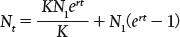
Note that N_t depends on both K and r (e is Euler’s number, a constant used in natural logarithms and approximately equal to 2.718).

Figure 46.5: Logistic growth in a population. The graph shows the characteristic S-shaped growth curve, which is determined by r and K.

Logistic growth curves, then, are S shaped because they actually reflect two sets of processes, each related to population size. At first, growth reflects only the rate at which individuals can reproduce themselves, so the curve rises steeply. The second part of the curve, where it starts to level off, reflects the onset of additional factors that become important above a certain population size, such as decreasing availability of food and space.

Virtually all natural populations grow this way. Logistic curves also apply to many other phenomena in biology, as well as in chemistry and such diverse fields as sociology, political science, and economics. Logistic growth therefore is a mathematical concept worth knowing. For example, a logistic curve describes the rate of binding of oxygen to a population of hemoglobin molecules, as seen in Chapter 39. Similarly, the number of fertilized salmon eggs goes up with the amount of sperm (which reflects the number of males in the population) deposited in a stream by males but slows again as the percentage of unfertilized eggs available for the sperm to fertilize drops.

46.1.4 Factors that influence population growth can be dependent on or independent of its density.

In the preceding discussion, the factors that limit population size depended on the density of the population. At low density, food and other resources do not limit growth, but as density increases, they exert more and more influence on population growth, spurring competition for available resources. Similarly, at high population density, individuals may be more vulnerable to predation or to infection. Factors such as resources and predation are called density-dependent factors.

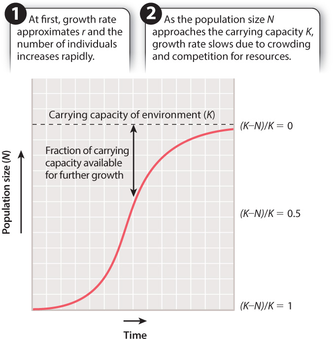
Not all changes in population growth rates result from population density, however. Density-independent factors influence population size without regard for the population’s density. They include events like severe drought or a prolonged cold period, either of which can cause widespread mortality independent of population density. A graph of density-independent effects on populations would show instantaneous, rather than gradual, drops in population size, and these changes would occur at different starting densities.

For example, population growth in Song Sparrows is a function of the number of nesting territories established by males each year, and of their young’s success in those territories. Fig. 46.6 shows that the number of territories generally increases for several years until an unusually dry spring occurs, which greatly decreases the amount of vegetation available to support the insects on which the sparrows feed. The number of territories then plummets, regardless of territory numbers the previous year.

Figure 46.6: Density-independent effects on population size. Independent of population density, extreme weather (such as drought) lowers the quality of habitat for Song Sparrows, reducing the number of territories occupied.

46.1.5 Ecologists estimate population size and density by sampling.

Imagine trying to calculate the growth rate of a population of Lime Swallowtails by counting every individual in the Dominican Republic. The task is hopeless. Like that of the Lime Swallowtail, the populations of most species are either too large or too widely dispersed for every individual to be counted. Instead, biologists estimate population size by taking repeated samples of a population and from these samples estimating the total number of individuals and their density. Because of the importance of population size in ecology, biologists have developed a number of sophisticated sampling strategies.

For sessile, or sedentary, organisms like milkweeds in a field or barnacles on a rocky beach, ecologists commonly lay a rope across the area of interest and count every individual that touches it, or they throw a hoop and count the individuals inside it. Each such count gives one sample. In practice, ecologists take a number of samples and use them to estimate the number and distribution of individuals in the population. For example, suppose 1 m² hoops are placed in three different spots in a field, encircling respectively 4, 5, and 3 individual milkweeds. We can multiply the average number of individuals (in this case, 4) per 1 m² sample by the total square meters in the area of interest (in this case, the size of the entire field) to give an estimate of population size.

It is relatively easy to count sedentary organisms along a straight line or within a grid area, but many species move around. How do ecologists estimate population size for turtles in a pond, or mice in a forest? In these cases, a method called mark-and-recapture is useful. Biologists capture individuals, mark them in a way that doesn’t affect their function or behavior, release them back into the wild, and then capture a second set of individuals, some of which were previously marked.

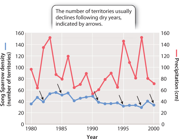
In Fig. 46.7, for example, an ecologist has marked a butterfly with a painted number, which does not hinder its activity in any way. Later, ecologists return to the area and capture another set of samples from the population. This second sample will most likely contain a few individuals who were captured the first time around, identifiable by the paint mark; these are the recaptures. The rest are newly caught individuals that have no paint mark. If a large number of butterflies are caught, marked, released, and then recaptured, it is possible to make an estimate of the total population by extrapolating from the proportion of the second sample that is marked.

FIG. 46.7: How many butterflies are there in a given population?

BACKGROUND Individuals in many populations of butterflies (and other animals) most often live and die within the patch of habitat where they were born. Population sizes of such animals can be estimated by a technique called mark-and-recapture, in which organisms are captured and released on two successive days. We assume that the population size is about the same on the second day as the first day. We also assume that the captured and released animals mixed with the population and do not avoid recapture on the second day.

METHOD Butterflies, such as the Karner Blue Butterfly, are captured in an area, marked with a spot or identification number on the wing as shown here, and then released. The number of marked butterflies is recorded. The next day, butterflies are caught and the number of marked and unmarked butterflies is recorded. Butterflies with marks are the recaptures.

RESULTS To find the population size (N), we take the total number of marked butterflies and unmarked butterflies caught on the second day (C) and divide by the number of recaptures (R). We multiply this number by the number of butterflies marked on the first day (M), as follows:

N = C/R × M

CONCLUSION Let’s say we capture 100 butterflies on the first day, mark them, and release them. On the second day, we capture 120 butterflies, 30 of which are marked and the rest unmarked. We conclude that the population size is (120/30) x 100, or 400 butterflies total in the population sampled.

RELATED METHODS Mark-and-recapture techniques have proved extremely useful in estimating population sizes of organisms from polar bears to disease victims. There are refinements to the mark-and-recapture approach that take into account the movement of individuals between populations; these methods involve taking multiple samples and adding variables to the equation. Many animals have distinctive color markings, such as the blotches on humpback whale tailfins and frog skin-spotting, and so can be recorded without having to be marked.

SOURCE Lincoln, F.C. 1930. “Calculating waterfowl abundance on the basis of banding returns.” Cir. U.S. Department of Agriculture 118 :1–4.

These methods are simple, and they make a number of assumptions about the population. For example, we assume that the population has not changed in size between our first and second samples. Nonetheless, mark-and-recapture methods have proved effective in estimating the sizes of populations in nature. More sophisticated analyses are available for more complicated situations, for example when more than two samples are caught, or when immigration or emigration occurs during the time between samples.