Chapter 1. Mirror Experiment Activity 45.10

Mirror Experiment Activity 45.10

The experiment described below explored the same concepts as the one described in Figure 45.10 in the textbook. Read the description of the experiment and answer the questions below the description to practice interpreting data and understanding experimental design.

Mirror Experiment activities practice skills described in the brief Experiment and Data Analysis Primers, which can be found by clicking on the “Resources” button on the upper right of your LaunchPad homepage. Certain questions in this activity draw on concepts described in the Data and Data Presentation and Statistics primers. Click on the “Key Terms” buttons to see definitions of terms used in the question, and click on the “Primer Section” button to pull up a relevant section from the primer.

Experiment

Background

From Fig. 45.10, you have learned that individual insects are capable of learning; a single female digger wasp can learn to associate certain landmarks with the location of her burrow. But what about insects that form colonies composed of hundreds or thousands of individuals, such as bees and ants? Is any individual within an insect colony capable of learning, and do different types of individuals in a colony (i.e., workers, queens, etc.) demonstrate different learning abilities?

Hypothesis

A bee colony is established by a single queen, who performs all hive duties as worker bees mature. As the colony grows, worker bees take over hive responsibilities, which include finding food. Due to the fact that hive survival is dependent on the queen and a handful of initial worker bees, Lisa Evans and Nigel Raine hypothesized that these “starter” bees would be remarkably fast learners; both the queen and workers would quickly learn which types of flowers provided the most abundant food sources. Researchers also predicted that as a bee colony matures and grows in size, the learning rates of hive members might change. It was possible that later worker bees would be faster learners than their predecessors.

Experiment

Evans and Raine grew bee colonies within a laboratory setting, introducing individual queen bees into “nest boxes” (the typical wooden boxes you might have seen beekeepers use). These queens and the worker bees they produced were allowed to collect food from an enclosed area, where researchers had constructed plastic flowers. The plastic flowers came in two varieties: Blue flowers that did not provide any food reward, and yellow flowers that provided a food reward in the form of a sucrose solution. Researchers then evaluated whether bees could learn to associate yellow flowers with a food source, and determined if learning rates differed between queen bees and worker bees. Evans and Raine also compared the learning rates of worker bees hatched at different time points in a hive’s development (i.e., when the colony was first established and as the colony grew over several months).

Results

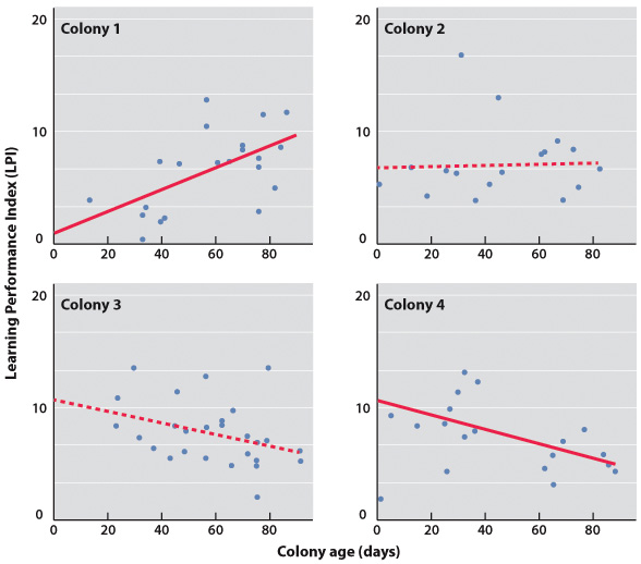
Researchers determined that differences did exist in the learning rates of different types of bees within a hive: a queen bee typically learned much faster than her workers. However, the learning rates of progressively-added worker bees did not appear to consistently increase or decrease as a bee colony matured.

Source

Evans, L. J., Raine, N. E., 2014. Changes in Learning and Foraging Behaviour within Developing Bumble Bee (Bombus terrestris) Colonies. PLoS One. 9, e90556.

Question

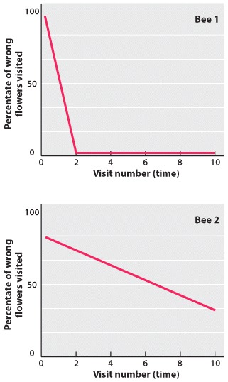
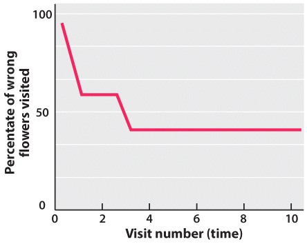
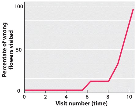
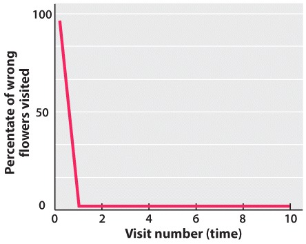
As part of their experiments, Evans and Raine generated learning curves
for each of the bees they studied, which depicted the rates at which bees learned.
To generate these graphs, researchers used ten data points, where each data point
was defined by how many “wrong” flowers(i.e., blue flowers without a food reward)
a bee landed on out of a total of ten flowers. Scientists let bees feed in ten
sequential visits to the area containing blue and yellow plastic flowers; they
wanted to determine if, in each sequential visit, bees landed on fewer blue
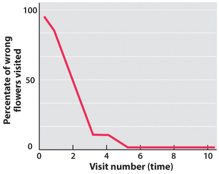
flowers. Imagine that researchers gathered the following data for a queen bee,
and plotted this data with the percentage of wrong flowers on the Y-axis and
the visit number on the X-axis. Which of the below learning curve graphs best
represents the data for this queen bee?

Data points
Graph A
Graph B
Graph C
Graph D
i1UMAGwf+lVNsLpRsYI5LLnCaD+kHNisiLjA6t9ioLDZIm56BbZ+6gBkrzfBZXrsi1O/jknoB+yhOklyiltUbqfWyJZlGa2dsnDJ0WPMzuT+8LJy9OXZ7PLcePNvh9bOArlRbJ22rLXUOdJRJGVZvjaOXCxj8c1EPaX5qyp6Gb4+pIaQJZKWrPx/57QqsE0BxIOLIxMR4CuTAxme5ezGO9A0rZPkG9Q+IuL3tJbKV1AYodSllg/0cCWg3sb01TcsuO7Jtw+rOXgqIPNeFW1Ii6pjBiwUBMARG0wtxspupkBIBp5mtIzL7Pqp4eZDDuBuYb9f2bLd+uOIJ8JpvXeXQcYOzX32U/Vo8+qu2HenDMzbtkZI4KXYMjj3dcn9lmdgG6W69qfkGf9ayiSxqt0xG13DYlrXMjhlzdTnFpk4ugmBoShgyic6+p277IllL8ST7h+NjkSfoemtqMghW3IXycyifZ3C+rJdUrBEZalsNX3m+a4DzhMATr1y3fLHfHyfGdnuJ3uBhEc5QK4hSbkwYNHZDM4nCJuuQGeuuN4ooaN87/hG2zmtFdmat/xQSQLHrhN11vfXH2w4MXVYOjLpk7/UkdUwCuUJgat/FhLD9p+uw7pbnR3P/tePUyBE2db5x5nvUzzO4Ghgk0td/aeP3jp4AiRCxRrmWKDYajZIOQ3lj0t4BxBSI8J/AVKvovsR1UvyXiggwx0pbMUYPfKoJSwH3vYTp53+b8W64Vp40C0p9Jvp9heDorOj+AVqKf48JxqkMmU6/43XTeueD23mhgyEJUEOgvuqc+9KBjafI0eIiXOV0uwsjRf08dnP+9kzyYo0qceKWlUKmFRifTQdx5TPbitLmb/TEr9+uY53H7Ja6ra3qFOxU9KrtRvgROr6n1dn85wAL2aQ9rTxbVN2bw==

Data and Data Presentation

Graphing Data

Figure 1

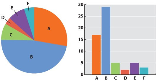
Now we can be confident that our numbers are reliable. The next challenge is to present the data. Typically we do this with a graph. Different kinds of data lend themselves to different kinds of graphs. Our mammal species data is discrete—we have clear categories: A, B, C, D, E, and F. For discrete data, either a pie chart or a bar graph would be appropriate. A pie chart divides a circle into “cake slices,” each representing the proportion of the total contributed by a particular category. In our trapping study, we have a total of 61 animals, so the slice representing species A will make an angle at the center of the pie of 17/61 x 360 = 100°. A bar graph represents the frequency of each species as a column whose height is proportional to frequency.

Fig. 1

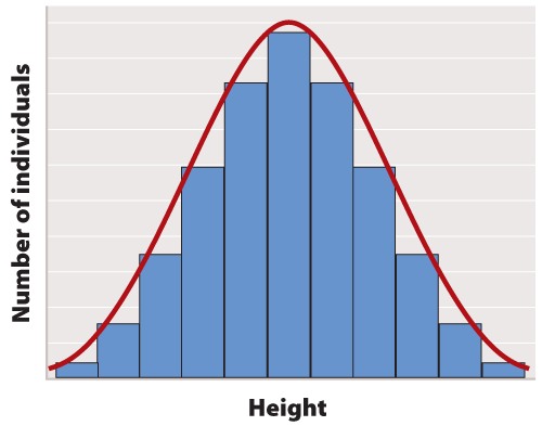
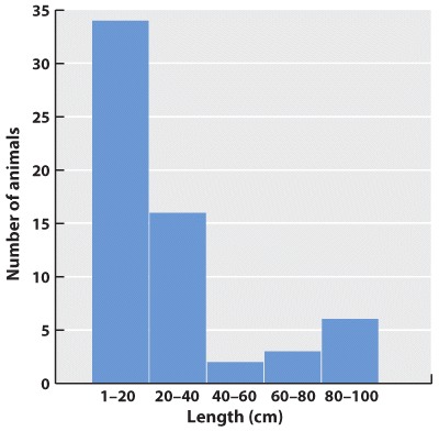
What about continuous data? Imagine that the data we collected is the body lengths of the mammals we trapped. In this case, we might choose a histogram, which looks similar to a bar chart; only here we have to impose our own categories on a continuum of data. Because they were discrete categories—different species—the columns in the bar graph may have gaps between them. In the histogram, by contrast, there are no gaps between the columns because the end of one range (1–20cm) is continuous with the beginning of the next (20–40cm).

Fig. 2

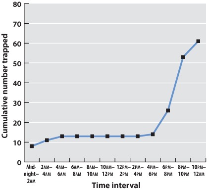
Often we are plotting two variables against each other. If, for example, we record the time of day that each mammal is trapped, we can plot the total number of mammals trapped over the course of the 24-hour period.

Midnight–2am 2am–4am 4am–6am 6am–8am 8am–10am 10am–12am 12am–2pm 2pm–4pm 4pm–6pm 6pm–8pm 8pm–10pm 10pm–midnight
Number trapped 8 3 2 0 0 0 0 0 1 22 17 8
Cumulative number 8 11 13 13 13 13 13 13 14 36 53 61
Table

Often one variable is independent—time, for example, will elapse regardless of the mammal count. We plot this on the x-axis, the horizontal axis of the graph. The dependent variable—the values that vary as a function of the independent variable (in this case, time of day)—is plotted on the y-axis, the vertical axis of the graph. If there is reason to believe that consecutive measurements are related to each other, points can be connected to each other by a line. Plotting our data on a graph using the values of the independent and dependent variables as coordinates gives us a line graph. This is a good way to identify trends and patterns in data. Here we can see that the mammals in our forest plot tend to be inactive (and therefore unlikely to be trapped) during daylight hours.

Fig. 3

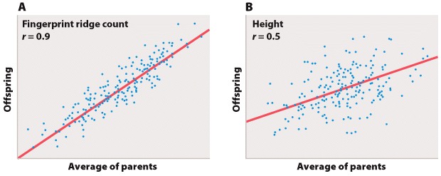
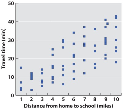
In science, data are typically presented as a scatterplot, in which points are specified by their (x,y) coordinates. Points are not joined to each other by lines unless there are specified connections among them. Here, plotted in a way similar to the line graph (with the independent variable on the x-axis) is a scatterplot showing the time taken to drive from home to campus for a large number of students. The independent variable is the distance traveled; the dependent variable is travel time because the distances are fixed but travel times vary. Overall, there is a positive correlation between travel time and distance (the further you live from campus, the longer, on average, it will take you to get there), but there is plenty of variation as well. Look at the eight points representing the eight students who live five miles from campus. The variation we see in travel time (from 6 minutes to 30 minutes) is a reflection of differences in driving speed, traffic conditions, and route.

Fig. 4

What if there are more than two variables? Three-dimensional plots can be informative (but can also cause the reader headaches). A popular modern solution to this problem is a so-called temperature plot, in which the third dimension is represented in two dimensions through color: red (hot) for a strong effect in the third dimension and blue (cool) for a weak effect.

Graphs are the mainstay of scientific presentation, but you will see many other ways of presenting data in your textbook. For example, studies showing how different genes interact with each other in the course of development are often illustrated using network diagrams that give the reader a direct sense of the “connectedness” of a particular gene (or node). Evolutionary trees reveal the branching pattern of evolution with species that are closely related having a more recent common ancestor than those that are more distantly related.

Methods of presenting data in science are not limited, even in textbooks, by standard approaches. The popular press has developed many graphics-intense ways of presenting data. Think of an electoral map after an election. You can view information on a number of levels: whether the state is red or blue, the name of the election winner, the size of his or her majority, and so on. Scientists are learning that they too can package information in ways that are simultaneously informative and attractive.

Correct.
Incorrect.

Question

dw5E0L6BXgFoH0HBQ3ZjGZSOD/taLGspOfHS2xdhqiZD7xaxKWgHxSRjwZI7uT7EC8qH5qa03lphedM1dRl/LWR7aPnsQWswkd8fMKEqxwXN4vxORO+g3lJvCgZ/9FUiglbz0cQH4h1GiMMVSeewcNl3s4drrBEMb+CDwKBKjDzrucUJbn+MPvmHqEzdlFrbhNMLef3z5QtgJjM9gbk/F7ZJeQ4fKI8K8myScVNMxLGugKrVR5awiZMvsUsJfHTl6rv4yl4zOJqCCYwx+tW78QPxGxQ4UOVoXdYN9mSlX4E/y7WXmDspo4INoheOq8fH/K7wuLa1YaEDgoZwiEVxmwZfzvfjdN+48xrSNaGBz4v7W/A1OBlMflkzsSfS4zVSJRtG5bd6d07OT2iwSY2tCDuX+yijsE+fy8XxXplwZBAsVGogl/Vf8No6Ij0Vg7upH9kGP4mgAoWlai8+FWtOmvK4g7kUHoi2Mql1UhSNbE0SKkw8wNG22CsFN9tnRJZa+F3K9z4Md46KHw3oaoFm1eWl6iSpBHH6rWn/h/i+soIXVDBY/xj6gaOfTliTfRldPRqLrr0Qh54wrT+vM3AsIyCDW1MC1WpzaizmG990Ig+qCZkiuqOMzjydb3sl/UsWGpeiXniLB2807egPzj7BQDCXvwkDdW5l9n0t5K6Mn7c+DpXePLUw9kdXUpQHkYZJUNO7u56QSs85Y8im2VVn0f/BdpKySUznBFewTbvxm52rRv35cWlwCCeOb3/kZzGOiPBZ9oJJ12MMfNsuuA6W03kLE+dAHzl9C4DPEw7hOCklD4j7VvKEO0ZSqAO01uBUh1t5vCxlvbQKeHmLqKTJY4AWCvZTXibhTUJ7/+Q5zBt1zAvDKfVGRU7pIpPEzCIuOjec6/6PEMn/YY1/PjO14xVViMjH7M0pObA8ihAliDRQSpcWf9jGp7N21p9z0sJgJe73pigw6Fri6sqJdC5Sai+PkPFDtHah0XVqJD2iopoGWRtuCrXTOVlcZJ1MYWXaTawetDUvqa1QI6G9Rgy/H9vDfF6MI+FnxbUr7mpW+6dZXiRndUXXcvutAxKzzjGVjTL6fCLdsKZcycESlb3GxmeufZ4DyreIZpMMyTFMbQe+68G973s87tX6dxQGPvIflh5PR8lFkMmH0GMJhbMuCfkgf+eh46qDzh6k/xKPSyOv7rekcW6z23NtXFEg67KctxLYe9cn1dLNPOiRM+EGgUVM4yETplADkoabyFK0M9Qg9aT4qgl3sLMdeHRnbxfhcH7ZK8bnie2b8yuVbVctqnr4UmiUlkK7lKAlzVsMT9VOFvhLXqywGM3/ouVDy6JpbglVuLADHxjsu0hDQH9LmJ2EQ9dJOoPiDPZYCvOs8LFHQ4p1o//b/IqMsrynhudKi2M94j7mXE4mYWrPLC5EyvEaiX44Sx2XJP9Y3bKNE2lylmA6a0qbIhD5uwajVR7dJiNJVobgilx3Znk/PA0f6c+QmJ8NUeCUTdbJ+Yg5xQcRV+SNPcspCqT9ClKGqwS7hmkrBsjvQZCyL23cxAtTuoNAidKdHmOsWnzGyXDyY3oZiZii0TSucqQBmPzVp1A/wF7SwlNAtTkilKSUYBwAi2rBugH6b4TuwRaOain4e0pzhwjRukg+n5sppa38lmk1tM/0f8ZoLdm5iNuCsvxOFlgfGGeVKqmJWi3I9RV49z/LwjavGTZBqZzcIpQyr8Y9LS1P75mGJcxhGfPuiFTerLu6o1MckqoBUKXx6Vcatjer8XGlSqOSogGc9ZgTPm7TlTPB+oKLvVFCSJDNdPB5oWE+DVRY/AcoFTmWQEr+YDHL+zTqjR1r3I7wyABP2AyGvqk4/bX7K7FqXY4jH6X2kS47y+rzpR/3JdxjLurtieaI8ykGrlefvgQtEAwdtfjap9h0xI40221XO5Rh+GStzoLOOL64kHO7pWqHETs+U7EgRjQsBPoor/ItwTfgzAAp1gI1Ldk9rHQopC+7TKDtJZAMSlYW9Wvx4XCRQKIg+RZJT6ASL3nxYVnwY6OqSEdGDmKYT39o1APtL7oTB12VZDbEfrftMrV8zwEq6u967Dg77xmHMUjVghNMjjzfvtj865iPSkxwVJfWLBWS
Learning curves
Correct.
Incorrect.

Question

mz6NEsT0u7Iwvv2FrT8c1EYYGP/PbrLWJh2vWjZcxc0Z19756+EVZH1V/Apnj8vuJfxOrtZ1vQ1HYeKioII0IHbWVWZoHcswPAQCciS8IXY7aU6ZPDei2aqJ/ar1IP3shkWJCOl+SJDRK/WQfinFXTojhlDaHeIGdBqF8OXU7O4TxYU56Mufxt/ZSyve1HylvvZ2j48ndhecv84LM8I6QNBKrxMZUSQUQLaH2iPej7I2LGJ2iF0yM83PNq6G7moB+FrAFdGDgQNHjeNfRE2zHnN7qENskK0dpx8edZmJP6uu0OVEj4cD5yUNCsZ4/3fAsh6Y4iP+ejDhYnftFAEKe5vxNMoUfjrGAS1t9taf18U5e/STclVkzorDywiMe4GFDrHPG9yge6umXCqpevFuaoOktfEGvzYT6eh6ppBDE8q2rfUts9d4P5hjkYlg2aSjE4j61vY7S3mzdZxrOU49VL6FU0NNHxvan86fDhVzWN83VOG083ST+5rWWkCC62+HSTadsZiTsd6d5J3Z3sCi9Q457BJh2IWk6MgWxtmpItwYw5OM6VJgDswIJ6Cq0q8OLVtRs0dL6CoTnWhNfhKR3BQ4Pyc247UzpI3/KFKCgMyITN1sopEXFyOKXYRxBKSMjn3NOlvDmEvL+G9pTXdXO0K03sunzkVXt0aucOTyItqJcLfEbOnlyNpWHDuWwqGOhapoQ3hK5LLNItWK3lgQxj5KvyUAlAauJs6ePbEccBU6W+2c69RCpM8CMNoHWxqmxp9rVHHs+AClhosrhi5kYITeuEu42vwzWend2Ds91gBfuwnSHtoiZxp/wGugJ3fXtAI5AIEaj0JW5z2meWirGMXfoZO+smjdJ93zKDTrGRUcHKCz9IW9fThqQiqRW9HsrKgdbFXRf33XxB+8Ux36+6RFNiUAP3HqYEJZrwrNaZrY0/s+8TdZ6QbaaU9hAOAylFqfY2jxr4hH3UE2JhKzTu4njdPIbnH0sa6S533e58sTBOH8X0V/NwPoSozpJ2zIL3jOP49gA70PoRH+yRMLyaHQVAIuOZiiybxQq/BOcC/GobgZCM3Sio0zf4L45r1pSnqFndDZYPwgfBeJdUfphTAUmIX+VBMfF4u1nA27NgTsSwC3PSb0GGv3u4K+MZd1CWTPNsGj+JWdB5bvwupHSgKgCxBli2t1om6XdZoKeEy+4v1QbhDp+6iOFLqAi0zkxex1zmcQnAo1usTHjKayH8DoH8bZO1cYksrKuAMRoc2dHW1JHWvQyMS+n8b87LyuSqkaMsFYQIQdHd50KsP48x6Bv+lFZ9/E57a/xIyQDuMoib3QUYphDKcvw5KukJB5KsabLvqdC0nxnWh+HD87mPEVSnDI8x4uYbSpXWLVKSEiYqvOZoxVPwfr0cgHOCyPshxUcHx0W330cgWcfmCWYxJy07b4tukBYHtFc5nwPVYPqaUKYRk3XTgdNx9mkx43QP3QgFyRk1NarKKbloXDOmRb/Enim3ppBKpZ92N7xD5cttWErF5wyalCf4YOIGYLgBhLNuM/T6qPKkUPGWemD6K0/9O+nYmtyKDOhPwlnMgWZLOSzKp4Z02q9pAMbpIFXzXoD6LgOqfRwteExPHRP2vFKq4LCSA37tPsKCYoGan9sYtdce2o8FphVhvQ7SJMTh0hG0+HDmzR9DR/U6CaLKkn30xQqTKCxPKeIiocvJn4H880CssFinuo/lBSpoUYmnCRXL27w+kSutlq+gpU9cd8gIcpYFfQ9QJiEr3tQov0BggVFQ0jIWq5lZqia7SfjLkxqu7N3XzKAo1YXZTpe0PKCkMpA+u/xDMirzjNeC+3KP5C+NJ7rdhcX0sotP75EG+XzMMRy+FdL3xdtYRpGg2cfBCfzBdHlmvf4logFAhUmAa+xQNb++FRmIfzAyDI9DWOfmH3NQQDuOGgmzj3KvtAyoFm22FeGnt1QGjfPcAGF9yxqq7aVDfY0Magi+7/6OJJEQGijPuSnGyrPcvARAG4eI3FDHCz2PLw/rEH0R/GxuAnuxsdFXfWMKmSn3A4PbhDtM8EebsUzRDdMQ8/b+qIHrgRBM8HpG6KIEBRKoBVnDlMMGoIKie0m1VPeFMmEHLZZdiORLd0Ip0CryucChcxfNJpKhlcJJcC5NRPAHvAHb1n
Correct.
Incorrect.

Question

GW7qcd/a61pJlttAqZxPDJn+QsciYYzLRN3DyXc3DkjlM0UT/KD2QawIpdvJwkzV99RugssAk1WHAP1sE5DkgZ9z547pQKC9sbk1ziVqQCttZYKttwwmMZEq1je/vzibzJ4hVzmkYnlAh44eFT+Rt+DwrGXSM3ds9/XmEj1Pk4Wh7gsFA7uG1FMdfkCACWGN5iaa9NoaR9UuzDUEs5YtAQxdwI8Cv83i2OEOn5dpmwvRSI5eZmwbf3U9QhDzA8dujz2IQgnUjFHWqk3w344ciVdnwVF+BaUADKz0lbyyTSpaAMOpekw49OXXTNADivXTopMydCjBS1XU0xcexoDgeFjbcCPu4VveBVuXcXeSIQmiwOJ4ZJjQWrj4mjE7q0XQE0awRRnsPZ3oqXJ3DATgx1858IcGQ0dnhv1DLvollnSyJKZTfHAh5VcVQK1Cmf26o+DFCA2plQeFN8CKrSdkv3jA7tZFZTe07hZND+tTwMaC3GWHGlBbpWS9883/TRBOAtGPvaqhdqboz7QbHqu68QfZ8bIAboV/V36t37sRCdg8h9WNDtCqpSXPdK2nOBm0a1kpJV0QAx7eMXr4ZhB7ty6lsiG+I5r5RGrYaXoIrGscGCZpTqf5m/Ap20MWYDcMknCKFoPnb4ndvvwYvHzhpcPkJXVuTKXrSy+Q/mH3PlS2s4+Y+iGrRAitBTtTFoUqmDHQY98OXG3rCOPUHpcEH+P+1oqy1QgL4u8bCO3xnKwDp+71AZrXC1tl1FB42IRpwNjjMxxhHrMvdPXvs5dl1wmQD27f1KGZQvxW/wy4GEKZakKmIG4QIe/dqkO/vJ+pPBAvwbx6FzyOOMAWZ75JpH/0dQiEiMwws++NLz1/zynJijHwP5QAIjjEQbXi5Ojvas7SSi9alRvB7uuGiZ73LVgCTd+Fe/0I6tpwttEjUtw4LD7CFvx8pIc964191tWMD4Cv+Zt2hmLVSm34DtVH2Ga+3uHgWOvN9qpKDwyhE2TqQRc27I3gJp4nfn0OwK8/h9vr/YnZdeMWDFO0BvC/WKnMu/mQv7OKkMhSjOdkbajWu6yVq7bfjI5Aoq9SP+r/Wb+WRShAzVFh7UuA0SZb9PSS9rUPuy6Zkk/ct7WVgY/1bxUaK3SdPnt7JJI3NPXB57iahigBVW8PphM66ZuRyIPWVxTAphOuMPWfD3CEZDNxB/WYShhP2wlDO952Gw7ve33IhzJLeuzwBfqV1jvDJ3MrN/RO3w+D2fcelrlNTWUTpHwEiXAD6FkqOmgg9DCRxNaeZFueuBah6pusrmziZTkHnpdIeuvNptEqukkuJHM4g23i5xWqbUZUWbZBi6Hq0gj2z0oOPUy02sRbLZcX84Hiny3pfspDt0oYh+XlSUCPwC9YHt0lsOvqvtBJYBg+8dlYF5UWZEB++rSeCJVI4MMc4yTiQHkEJsioV6Yv6uZfnXz80JLrdR5JVn245qjVd792klQxqDPImo787wEg5aczKgRkfVbRkkOLw2+2npjsS8r9LuqQ1nFRxRvMCxm/RN7wk3O+GPST+D0QPOptwHtCKepjbSzRePX/N8ycX5rLXsNgiUGEcH0fn/nJoBSGsFOxrmgQsKf8NvQtfhfForidXQDiqhw0dNsewi7Wh++AEaOu/1TeSP77GU2jhWZm68oxUTarMaYcccIf
Correct.
Incorrect.

Question

After creating learning curves for each of the bees in their study, Evans and Raine assigned each bee a “learning performance index” or “LPI,” which was designed to indicate three things: whether a bee learned more when it was young or old, how quickly a bee learned, and how much a bee learned over the course of its lifetime. Although the actual equation used to calculate the LPI is rather complex, researchers noted that the higher the LPI of a bee, the slower it learned. Researchers collected the following LPIs for queen and worker bees (an excerpt of the actual data presented in Table 1 of their paper). Note that here, queen and worker LPIs depicted in the same row are collected from bees belonging to the same colony. What could Evans and Raine have concluded from this data?

Table : LPI
Queen Worker
†0 6.8 (±0.72)
5.24 7 (±0.91)
- 7.6 (±0.57)
1.29 7.2 (±0.71)
1.34 -

LPI

lab71GOA8yoy8DY5m5LWkk5FYplnkmCW0hoZPnOrzbu7yrIjI6L3sdfO1hU2raRF0r1eNvAl7zCiOLlOpdlQ1k+B7B/9G4lcPKuUmwz/jpz4b0zyw6de1TdhDy+VcwyCBEE6/lM2GspX7bHM8bbOvX+idbwKiQozAtINuzEadS8tGBAgHXYbxFi9lntp4AruMhfK5nEZ5PlpNKszLHQscl44MYt3IsNdKYxuFXkATk7Y6N0BMpkK12TG1K1SP+C/jnax46G7ZXvXfbXwsUEY42ar6zf+dRFc7DAFeSI3taY5XyOERc2XpUB1fIxT/uYSMIyMqUXU0AAB1nlBi0FbcBN/ZyOqvM81N2o4MQgg3lKz9b+bPUQV1tP48/5xlQ3boTwSbE1t20V/FwHKY/zi6XnbAprRaY4Z7zJEDs8pLzDZgHaQhWSqkUWvPo03U25v9xCvfv1RFK8bFy9ZvEQ24IEiRc/wKS9hss49khRgMFHgTDWQIu4rDmWmxUVabikgDLqglKsyad2rTaDkvQf8dE4Zsq0ozKPRiPAwcH80JhiL8y5YWUNn17cLDBTq1AgHk/EnM+YVyFz+libwKHWZPfox01bkhdUTAmfByIDHxv5JOz0kzWTFNy8f/6Afsnw1Qo4DH7NlF3L4oSrqreudLLCK5XclSu8i+GFCq42bLk6RJdbHD34Gyu8yxHH7MfkIDxp3UTJjKTGjSPQId+ZyDWoes2eFxLsgb3mEujL318hMBNzBXy01IDmVAjmLVwf+mfgbfc0ADsQT2m1J9LtIpYXAQRBVzEyr//OkypB8/qtm8ivOKyz9aYfjSC+0X5z8nFAzD+NWpkwYV0SWZ7DEyhB6Tp+pTn4xau0BjqvuhgktCw0un/Bx9jXo1fT8qqCk227Rt6B3llWWI2bt96O+xnExURFi9ZNmBqSo3Yc0qzzFmjd7wsLeu6gN1cLjMdJQodDoMZdxDZjRjJVvA+LUQS3pzgw1YHTwtfn6euK3hFZ9lU4lhXXZPxFSGz/bQU1NiphczEkhi0gUDolqRTGfBKJxeW0RQ98VzrUg5Jtfn54qJSsEl41t5OqMKWe2MB5kwQtFKy/ZJDp3M5oaAfLJ2Luqxi+rMv1mJp/NX1aXzJtO7rWLPC68W9Loj11xGXKy9f3zClz3G4S9we7bQld+qtE5p3xVcLbpi+tiCsg4LNwMwZQ1mvbDbB1X6BmJTSKyqnj3nfq8L5RpQYZbrhCkbakmUkGB4z4hztW35q4+rnFyTWNRijDANjLiSDWU4UtZs3qw8J+mA+/m1mHY39IGU77e/ybXcDULbnoV2tmPihLEsCb8UeGfbthBbEytpAhlnsstAuRMCwyLq5u2pU4b2zBqIfbuIZIVTv0UP0Y6NHfSfI1cI7hYdbpyh8WtYxGRh/wyz5LM2vo=
Correct.
Incorrect.

Question

/Pk5A4U6faIKjUknSrper5oDGIFxN7ODEsZhsn0JrQofxjb2Lcy+Q7jfywWq5QoBONHbQjOwYr6jc+h7RMqwVXFeYZaXJgO1fp5TXeyiWvSewCsdhmI7R/8TdO+y3JghAfM5vLkchMRYSYI2AfJjJS+UHa0+FbeFMhRg3JQnliSG4+UFZ+tAmUd5f3CaKPb3TfD+zl2n+5fGlQ0TpACizML4hnh+69FyeK4MYmVKjujQXN38DqThAFddyFtTPd1NXAaK5Gy9uEZdINCPgS+wEgYvvmdMdnwXvL/Zq3st0U5GOQTwcOmUULGQgvPjmNxRhREBzb9E9oPXYnf/lXlcoLyG7mex2BnT1+dSLVKWc7+oOeismSXESe8FeyxDip4rrF3EwrphLE7vjhXD3WrNMGXRZOeKgtpt4ZL7DFLI4buK62lrxGIjt80EiSxAPlf4sw0o9qWse4lKBomPcigARBVg9jdIihTevTAU/CcdwLY63j4Qw9gVXUJjva67ECN+FMoyTLZimp9JZ4LRObMe83jScEzEcwAQo5IYUYuvMRYHs1uBb6i8DPtNlYdme9L5sd0kE8nbxTwuLN8Hg4W0joGw2EDiSbEjullilnMGlYPlwjPk+4reaUEZ2m41gEEPbxEw0Oby+RUts6xpBjFtAnzcQw/QydyOQoBqndMhwKAXKF1rb98hadj9vFFaxjG35AJ2of1uzS6FTGjLdUYROOO/CG6xeqpcpm54lu2wNA2sop+j1smhLNtQbLtqtLD7LQ5sjaqACwZfg6s2YfgyfO9af8DpoH2WEkBR30FptPpNuaeTx3RHjSZ78CQkWw6slVKlKhE3MrytuZ4TflBfOW+rm7105J4+LFzRSssSGQltNit11Nky4qYC/wHXGGpsCFGPmKR4NR/i4nvXUf00LpfmO0ssyRyn0bEg5Sv2lnVCVEYgQZ4rqhbvBumzpxyHwk90UKYdWNEnygGy0r1BuqxoW5UJbTmBWzwEVUXfxfv78Zm8Xyi0vTla0In1N8BwVylloIXnwFfOH2PdJObRrSDPYhCE0gBVCK/bEDpdWyIXiBFc42nQN502ZIXdcVscmjFEabPuT2MpNXOv4Atq+Pdf4rNOR7klTSofefSFvIGHk7GJTb4hjQt65lNolBKD/mRgF4Hf5Fx+So5+YgmHteY/OGpqcGlQ/sKeO76D9STXxm7IYbnAxKj2lj1newVQTC/lHQoXuaeVREwqCz226on2fNG8brgdvTnPPxls+FzH4mFic55ufk3x17zGcp41XA+ov6s06B0UJcWVpotfVa65bgzmvYre4fPv/uqXojllYkAUHmBG2FtDr+wiO7I/THEiOZArGTDj+C1xjpfZC0w9Km0Q6HejnBpkJrg4Vd7kLL9Fgn4haW/sIQ2OC6ydqOTzcrnyHD18alZByoy/RnTWHC2m8wu2caQFy+7ZlOM/k65HhJNMtd/mDn+iqvIC9IYFXqyijSo=
Correct.
Incorrect.

Question

3q7YdtBUzDjBPVPPLP5sXTJq6buTFRtSeTWTAkP9B8s6ETJ6V6YCG2roPMrEXRud7FJsl+kZCDCE6krQ1B95VUtEcIpiw0JI3sG/zCcFSk3R5geKUw/nu+9u85ZRWiR9wcINLSvvyhaIzrzYnvrxdN2Ny3FsGith5PqvDrXICJDf4K4FJ6dyHB0R4DNXRUM4abBa4bnbI7Lb5JFAJ7NsUEx8Hj7jsXv5vDiIkURaU7Uu4SwvnInmyUWoRtR23lVv3ZPo/aguD0LhukSVV/nkQDGbgJUGEpaXHUdjk+DLXISt99xdyWv5axrlUt79guZrbHV22SgnSqmFFQTFj96vRzv0QsaQIQUw3s7AMb6y3whkxp5nslZ7JboLT3Lujiz99GXABbhk/HhajPIraCjMhZlW+dv3nQnh8GQ/LhTPzQLR4yxa4ddD1I1Hm/aiIXFlzkrQpWWODsujetSDN+jNVw0+YfZXxNJd+OI4da50j2QMnS8WtEbOpFFkdN9s/qOY5WmQhtGc+9T7qFXn2IUZao2HPLXu/t8gxanp+T4Xzg3HZiA4xp2I4ysniP84+NkSQ7c1pt3ngI/VIb9exb0LMuxZHz/e7xhoTkz6HCKhB2EITEQ3i6oZ/egxq/IATYYuvYU2ceh2lY0UWVfA2zK62yimCClDjEYrc4DZ1HWhI1KE6FMhPj2I0GM93NCgnZy4UbT7Jj70ALVpc2oEjMrw6DEw9nDsgzlbD/UoiKpmpvKPBB2tQJsCazX7YA9dF8VadzdgHykCRLohE687a2LQWEiZ06RmXdeegPwQ8CDQ76XEYyb2QPO8xfCJD5IKT4DKtSApy8pYbW5cOr98Xy6C1LIBDHTTGuW88Mmj29jGzFcAgjk9PZfmX4Lft7OvrkAiyHw8g7N90JOkCcRUil7KroCiN4NvmDRAq/MtlLeDmVanmUl634fo6wpjyq6R58UOD3lS2G/tSOognODFoIVtlgKLjHU4yEP00JhknHoOGaQmolo+utnsCu9ey340dHjX6+tBBWOBufMCA25eDoNYSZXqGPJIiQ/Y2QtvnVIa67Dr7Rm9sD+c7yRBFMHtmnGLu+mDv9BvaAhhHD57HHOQxPcAlRpnk2qS2xePrv3Huynfo4gf+ArPgULkfTRS/92RQepm1ueeXpenciK2gv3fvL9iCmCEIV1vpq7e+63xIHsOUQS9RHqbPwq92jKjGfx9Eb4fdIJqcGIvUumX5OVkZWm5oXUyUGWzC4RQUzdXfGUfvDfVN/zvPewyj+luXbj/plLuQCwg7Sr4X4FLVlqvEX4++gKF2FVZgF7jsGYDVgC+xnjZbGkr1CyE3T9fhrsJ0GBeE73GaLVmWHXvT3tPVZhBgr9GTu6ILNiIWAhfY9koAMrQwIfS1LpG1A3voia+QjyP8Pu/YqgMYO40ZYUhu9fAw59QZ3yAhx5G+9PaBRqzIIIV4dTNVSNvjxvDqfE5Rv5Vp6hHpo6Uok8RPTPnN2wMPDAyxwBupiLj8EnzDjcktTyLrX9JVpCyhNRgUsVGIZfdPjlPlpdCfgfr9BQ8dmhVvAYYyKzwDar6DS47yP/tzebUJkSzi/SuDp2I88tYEUHMaHXbwM6gxNVpHw8dwVj38UrfaPoBl5EA6/crMOlVeKmnYXiNfGB5GrJryfET9epis2EP4QP1sMnhlk05eXwJfTG/XcRPZCYJYLrkGzPMnPHrBfEMFyTa7dUf+a0mtz7WzNzm+8EkUm2lHl/MaCsiBzmW2J8VRWg9yReOQ25WZR4tR5AHmoZ6UtwgQW59FBzkpTEUJ00KK+6sVvz04Qq+bJEj/kHFFjWQKA1eaVOEvnOq26e+6nZiGZFzp2GdOn8sdy+Zk13G04FGMLIpoaXEPcsjrTR8ghKRT69NNR4EE/ooc16mVeMwRBgy/ftgPSZYUnRKc7jXsLyVn/F24iKi1bdWd1+oDqUG1/R7QrsFMFAipznK+JrzhwjxyXWURqxFmXBdJDB9xnFp/oNHXMgAVp1T1lhad74J1OIjY9qyKmlc+/BjB66BiiXWKkvWKabZDm2MINrQlovY3LM5BrjO1GZUEJ/BwWbwjlq02soQR/uKNeCeilqS6I8Ed24Cmi7sXhXL/JZfjpuo755uIirxeKC9OR9olL3dfd51D31Hq46s4zRjjb4cUuySRkK9Ql3ODvQfCJDf7KVV9lO97HKbzcw9NwSQ1fRknq09wRuKWK+43fFF6zkumGgj2RvAG7L++DM3N26gZJatHU+034hxkzCMS8cFY8hNE6Cm5DtVsnW0uRK3Cuo98XKYgJanIJVpb2O7ZSH02ThjV1tvRXUhAEuQoiv71FqgvlgU96MObeCV+FlbBKxSRu1Gct3zygKLbwhREOgX504JaYerNF8UGp6ftqJ97lOUt8HVVCfZ/pKzXP9q9g7fAYf+rwk+MFckUY5hRi3YgUc2QrSXLagBAX2lfAyKszEU0z5RtoO0yY18bgnAne0hQjmX6sU8wzihXRTTEnRChojV5f+Y24WIyHpx/Qmn7+knt02fb3tsDzPqxUTEsaLZZbYo/k3K6ZH5jUG0+Yt2oZYd4u9CFRJ86xh8XLBhU5EHfBl3x9X4CKjozSOqLaPGFlj1BFEBf3eAX7RWEcAFYiDC9ot5XeQw4g8HvX4jxe7GZcCzUA3x++h4kHnZ+LFok/pl4YoQ3Yojl1+gQhQLBdsL9lxEg3AJmWo5XnM8aWPJx1YvIZr+5RwFx0n9cL35xgowHfepuf2WRruD5s9adtZ9Hc9/yjikdP5hWhTc6g1OGWN7i5TBP1vUWbHn385q0KXwG570LqCgcJsFtlcHs/Quy6rMl1Z5k/C2dVt68LTdXl2tOt07O7rZkjSzGUPTU6racIy9+WlCoPAkFgyQZI5rawLAo+I0ivk1g9YwnhjQ2akjXXi7Wk86yQSA8U8dRvnF14/QBuEMFssWhm1n19V6/upmUGCH8T6FAHH63aIf6sUbooo6WbT+dSCkwePhljFSppmmS6S6+PsIdtUhyKBFOvLMpl7Ga6Qro9/V5GtwjydKchTFkNvVX6W7FvPdA/lguPLecvZTTOFLzMy61lsviii2Tr30JDBsilA3rW8r8CGzgG+tWER6yaRLeSIX7CJpjshki01WSb98a/JcJ8PtBGLG2+e4DFejsEL58GNlRqUSfeZytf1e/YQGmKxy0JckXEgbMzxNY6lh9TMviEJSkKztPCHgT2Nr+BYa2J7AjB8oO4gV/9pOJRvcxgVsc0qX/nsr6VW9gpw4ZguuIRHWSaWZWWPbDDuIBvQkXWXD4SdvVjLnhmw7lTHe3nxJhYgCVJzH6ZiUV0HbDKWUzrutRT5V2IHUVP1W2sf8PcmHLpSQkslNnzJ6Zdf62v9hOF5Ru7obaGt96fQraSvycUeAeExN8Z10NZRrKDPMkXFJeGK0RblW7/TSemaFevQefFEGIWJo0rlKKUStZ1uwhVtkTkyIhBi7apJwgfTY5VRrfpJFpXnh8GiHBBWy7BSS+ciI0TYMCNrC5HKV1Ed1ea4P1DYTHgDBW4LyG6aoqDC4mKru4ALrgH8dXwahuEIZB0FZ2kdRwrsj51ptFjadX3JFHQluTrdQ/d37y/XGr6n8uvcLLj8tRZccUPE50p1ZN20x8vO457h5IvY/ozXFQFKPvPUfOeqYRwhj1QmDwx+fUV7D55/HO8Cq34PvnHE2VZGTZ96e6ChDkoWLkbzbBxfkg6Zhz65KAESUY0L9j3Ntbgdb4yPnafwGAqlDctXQ+t6S87C07DBFUDON6WTgqdkI2f7Da+3T8WGgVIG4g0uJbDaHg6XYwqfH+5VLz5WCt871ISIHutEtpbbUY5HTQAa4dPGfrnbss2F5rIA/4MMxSMOhc7K4jcf9nT7o0nx3Z7BWqXWAJ/SQBclKHFciggJAgqg0fBoCWugAht4nm5ppcV5pXwJC2cQzdw1uPiozHok7smhrwyoRG7Nyp/W7GmrceqtVBeY1in8S9Hoh0aY5Impcm2+nC9c36IBtiRMxJpKaIGn55h/yrsCwRmRLfiKvZxgNBqy9sFPsTYYA0zzd3LxHHJNCQKdQsRHRWoCmzvkMojoSF0PQ28kX+JnbhXJzJ/8ROQ==

Regression line A line drawn on a scatterplot that depicts how, on average, the variable y changes as a function of the variable x across the whole set of data.
Table

Statistics

Correlation and Regression

Biologists often are also interested in the relation between two different measurements, such as height and weight or number of species on an island versus the size of the island. Such data are often depicted as a scatter plot (Figure 5), in which the magnitude of one variable is plotted along the x-axis and the other along the y-axis, each point representing one paired observation.

Figures 5a and 5b

Figure 5A is the sort of data that would correspond to fingerprint ridge count (the number of raised skin ridges lying between two reference points in each fingerprint). While the data show some scatter, the overall trend is evident. There is a very strong association between the average fingerprint ridge count of parents and that of their offspring. The strength of association between two variables can be measured by the correlation coefficient, which theoretically ranges between +1 and –1. A correlation coefficient of +1 means a perfect positive relation (as one variable increases, the other increases proportionally), and a correlation coefficient of –1 implies a perfect negative relation (as one variable increases, the other decreases proportionally). Correlation coefficients of +1 or –1 are rarely observed in real data. In the case of fingerprint ridge count, the correlation coefficient is 0.9, which implies that the average fingerprint ridge count of offspring is almost (but not quite) equal to that of the parents. For a complex trait, this is a remarkably strong correlation.

Figure 5B represents data that would correspond to adult height. The data exhibit greater scatter than in Figure 5A; however, there is still a fairly strong resemblance between parents and offspring. The correlation coefficient in this case is 0.5. This value means that, on average, the offspring height is approximately halfway between that of the average of the parents and the average of the population as a whole.

The illustrations in Figure 5A and 5B also emphasize one limitation of the correlation coefficient. The correlation coefficient measures the strength of a straight-line (linear) relation. A nonlinear relation (one curving upward or downward) between two variables could be quite strong, but the data might still show a weak correlation.

Each of the straight lines in Figure 5 is a regression line or, more precisely, a regression line of y on x. Each line depicts how, on average, the variable y changes as a function of the variable x across the whole set of data. The slope of the line tells you how many units y changes, on average, for a unit change in x. A slope of +1 implies that a one-unit change in x results in a one-unit change in y, and a slope of 0 implies that the value of x has no effect on the value of y. The slope of a straight line relating values of y to those of x is known as the regression coefficient.

Correct.
Incorrect.

Question

W2FjFwDcTq2g12l7eQ5JNIU+V0B9Da+0HSLWozTnbk+/qJCZgGzZMv0KgdSY3A7WBsvSxXG+ZnejStUkExmOvhDYSjPvXfyJNWYBGe7dEgqTourOR5vFjYfGRWDKq6saywDsjZR/cB+fDsdp5u7DT3JuOQzYUtEyEFvb9JnKhUxHhOee4Cu1a8fHaO3+sUc/1lx8pcGh0gg/zFnwwZXdCcQa7B6aqI35O7rJ+t/zng9I6MAwuIQ5V0caNWnmJEgx2zi1QKZHAKTtbF6FR8dQMfOCbVfDLWY+5LOZJ8GWco+mp9pG1KZ182CJJpdBovoz7DKSCm1zOhn4syPGK+GH1P5DLpa98qmsfi84jSq1szIEKCA8cnZhY64N46Mmbu7t8wNalXUW1NDh6uC4mdeplWyKvNjJjW87+2qEGA+0TLD6H1U70okhlamJl5Bht2OEPCHMDJLyNsWH67VHyUtjU06Rcdh/MhVYSmwQX7GJ5PgH2JLp5DHzPScBJ2RiC7ynhihm75eMFjNTX3cwYBQy+C9Q+leEKw9GMI7Mr1dZNfKb5buOBywvQZTtbsT07r7+hWMN8vo0GhCc9ncwJYcQn/1LxaJDHlVcHQg712ucjkTZqnIcXE/dFjxW5DB6t6UCm8jDyntR2SN3UpDXqtz0WD6kQyuZ02fCCSKYnicxz14XPz2RWKl7M5kLGmcKQeTtmKPaMhQOrdGrBf1dze/6dGd2rIjO8AS/gSugiwg39RGtyukDqlBpWpp3SWRYG4Xpb9dTN4WFrkgYknmNA/JpBp/olaFTk4RXfb7R7eXrDcB4kmjufLIqMIPL3vi7GhcoBlJ/NzATON3vcWS35tVc9zQ8Rs3t+Mqs7GRFLZbvgJYwpKXaHiXK3LAPaUw9T5auvXrtejgnIwP8FAds/s6A3jZKPebQ4JsjBG5SHn4pcICtJQoPHSNXKqxiMYWytIsayopuF9/f4kHRyZGYtDylFzlRtoYFhmZaDVUlzHfNU7IbLwOMGta6winTr10HThSkERwqgwKnjB3DmRHUyTnf4UcKo+RnuWq48LIqews1Cfz7/OShw0INvPCdnWkhFk6MUF8LRQUUo0sHBIY/x5pSLJSTBIgrziU7dk8TKTLAUMQyZs+GSojIUMACeohMNeG1g7xL9e/OjEvPU0AkImYn7cbGdWgvQGO+DG/zr0lbecRK7HDZhWXZYM893RJUC8/n1SsZoYdrmotKIbKa72YtnoGuzB9M4cg/MZMXlfu+RgMV24NhMqnGcdFyqORW4LUQzA43OrddA3M7eaEoZb+mX4r7xDcx0i1qYir/qGIIDc1ylOBl+rjJQZZf5WrQvGCOxXKtgROdVgONPCMcrpZKwl4ccHaR8Mk6tBhEwJN/3m/Y5op70JwJhb3eSPd8Q/yerjo3e3VjQ1WiRwENNecieQTqqUYw1R4/xeYhOdFzff4FVZeUPqmuv1S/V8bCAnW/jU4GMKu9xNhFiOGr6MIPzTTBxKaGxAsFlQ7cEst7S44DFWIQBU7/Tb/AAOtb6QL/opEX7yraf4LEUaHzDUqW79zwnwi5TCakVb7DD4jQNQAO/RfhqvXyRWAVnIM9DfuOvZrYhwFxQDERJ+RKadWHMBo/O+bmN4u9SBfIC0+iLmF2cQ/JyZcmNhb4Js8xlsUyAmple2t7hhSHQgMeYft1bBXH09Zt8sQcqt62ecDvSuFCIVUxetHmeeB6m7DpMOcW+4RQxUPeJl7fmw+DW3FXTJ2CA6anT9hPseGjp2mLiglFLtyzoD4++xhLgvbAp6haooWkyD6jll/3/t2AIng3NalZlLmrmZgqPMc2766BOBTGZJGkYuSnF0Lp3UvY6kNHYj8OKQ400Iml5lMgaOdbqOd6ZkGzp13lX968vRQOpUeQdqZVax5BdnaBIFeCr9roNf+MJWdB2DrXUXlnwBbYZDPo1nPKjEYkran9LSwNHa5CiEuxmsN0d8JeC6qgG8UzAwx8Ti+ab6k7TNgBUfTF6yseclW5weg7Nzsp3UQv8OIKwT7jXmEr1bbQ7RKhZt9twhHpHEzexvVpGKoWcFajIVJ/X2is5FhXXW15oOwZfhtkVOIXcsY6TxdEmam8gLpTaIZIuET9jOjEo7mRPZo4w1wkGhHyZgKnV9Ne2lbg3Ik1ip/GGoDuJySXy0wQpbm4vRUqwlWHEbC/5sApGGSLhcaAUhiOMYxKAK1gn1clgziN03DtvvkIv5vlFNR3WaU/lo7LeLjEQmswE1tLgMMn5lqj2jert2VGkeHr4V6WLIhrGpV5ItKvUeFvUb27RRZ/qV4V1T5dEyAHJCiVDGuulXyaPY1oJSzA2oGY+SEUpLoAkYVKTA07GdlGxm01RVwNjfPKS/IxejViKpf8TgFn+6om2CRRik/5E7ATlYEyqzRgCWaDtbJBPLZYcIyWDxTswoeHbasH+qDPjls3o9ut+6Qt/DPCDTgmPoEAbJ0MMQrk2WZfZPUpobI0/TnoQTjOMNjYqGiShAKHw3Fhq20A88X5fZCh4lh8Ew1f3L8ft4LaQ6wiz/B1XXN9Wq3S+aavEdQvtXLaPYepB0IShnd156XEdWYEklN8h5PerEFflZYDV99K
Correct.
Incorrect.