Chapter 1. Working With Data 16.14

Working with Data: HOW DO WE KNOW? Fig. 16.14

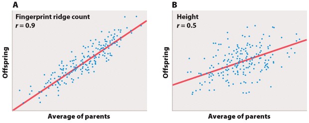
Fig. 16.14 describes the conclusions that Mendel drew after conducting numerous crosses between pea plants. Answer the questions after the figure to practice interpreting data and understanding experimental design. These questions refer to concepts that are explained in one of four brief data analysis primers--the primer called “Statistics.” You can find these primers by clicking on the button labeled “Resources” in the menu at the upper right on your main LaunchPad page. Within the following questions, click on “Primer Section” to read the relevant section from these primers. Click on “Key Terms” to see pop-up definitions of boldfaced terms.

HOW DO WE KNOW?

FIG. 16.14: How are simple traits inherited?

BACKGROUND The experiments of Gregor Mendel, carried out in the years 1856–1863, are among the most important in all of biology.

EXPERIMENT Mendel set out to improve upon previous research in heredity. He writes that “among all the numerous experiments made, not one has been carried out to such an extent and in such a way as to make it possible to determine the number of different forms under which the offspring of the hybrids appear, or to arrange these forms with certainty according to their separate generations, or definitely to ascertain their statistical relations.” By studying simple traits across several generations of crosses, Mendel observed how these traits were inherited.

RESULTS The “statistical relations” became very clear. Crosses between plants that were hybrids of a single trait displayed two phenotypes in a ratio of 3:1. Crosses between plants that were hybrids of two traits displayed four different phenotypes in a ratio of 9:3:3:1.

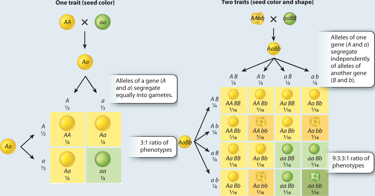
CONCLUSIONFrom observing these ratios among several different traits, Mendel made two key conclusions, now called Mendel’s laws:

  1. The principle of segregation states that individuals inherit two copies (alleles) of each gene, one from the mother and one from the father, and when the individual forms reproductive cells, the two copies separate (segregate) equally in the eggs or sperm.
  2. The principle of independent assortment states that the two copies of each gene segregate into gametes independently of the two copies of another gene.

FOLLOW-UP WORK Mendel’s work was ignored during his lifetime, and its importance was not recognized until 1900, 16 years after his death. The rediscovery marks the beginning of the modern science of genetics.

SOURCE Mendel’s paper in English is available at http://www.mendelweb.org/Mendel.html.

The numbers of yellow seeds and green seeds produced by 20 individual plants were reported by Mendel in the following data:

Plant number Number of pods Total seeds Average number of seeds per pod Proportion green seeds
1 8 57 7.1 0.21
2 6 36 6.0 0.31
3 6 35 5.8 0.23
4 6 39 6.5 0.18
5 3 31 10.3 0.23
6 2 19 9.5 0.26
7 3 29 9.7 0.34
8 8 97 2.1 0.28
9 6 43 7.2 0.26
10 6 37 6.2 0.35
11 4 32 8.0 0.19
12 3 26 8.7 0.23
13 10 112 11.2 0.21
14 7 45 6.4 0.29
15 4 32 8.0 0.31
16 7 53 7.6 0.17
17 5 34 6.8 0.18
18 8 64 8.0 0.22
19 4 32 8.0 0.22
20 8 62 7.8 0.29
Table

Question

ODtZ3oZs3EZugPb4qCI1+VGoMX4rIJ7wbughR6H50/OplagXus34Qt8ykiYA4hq/e02vzy7An++xJH8YSEHAbzvYT9U8oE6zMrT9HUGz5v5rlRIpjCRJmP/uw2UQ2NdcOJmXI9ZTtkjci8A/xFrA5dcDXdXp7SUaJySK7CCtfnbMwXloV5Rs0Ec1M2BxPJbOAfiKIHfKGiESThQHU/3TDOuhp0KpJxODFk9fVIZgeqAUr9PQYduYx3WeVtUEfWVLExoKZer1Sam/cC9vOwytucjelDD/iEo9IJJJYlRBzXBuxY6XKi2UeIHtHFghmboivrgfEfOf1YVpuY7BQQjTAH6QIZNrb0yDXsuJrnUdYyt5VizoQFc2dTizrHhA539OdqA6BJgEzfOPXmVi
Correct.
Incorrect.
Incorrect. Please try again.
1

mean The arithmetic average of all the measurements (all the measurements added together and the result divided by the number of measurements); the peak of a normal distribution along the x-axis.
standard deviation The extent to which most of the measurements are clustered near the mean. To obtain the standard deviation, you calculate the difference between each individual measurement and the mean, square the difference, add these squares across the entire sample, divide by n – 1, and take the square root of the result.
Table

Statistics

The Normal Distribution

Figure 1

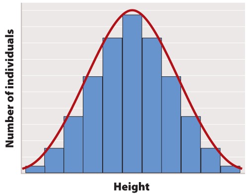
The first step in statistical analysis of data is usually to prepare some visual representation. In the case of height, this is easily done by grouping nearby heights together and plotting the result as a histogram like that shown in Figure 1. The smooth, bell-shaped curve approximating the histogram in Figure 1A is called the normal distribution. If you measured the height of more and more individuals, then you could make the width of each bar in the histogram narrower and narrower, and the shape of the histogram would gradually get closer and closer to the normal distribution.

Figure 2

The normal distribution does not arise by accident but is a consequence of a fundamental principle of statistics which states that when many independent factors act together to determine the magnitude of a trait, the resulting distribution of the trait is normal. Human height is one such trait because it results from the cumulative effect of many different genetic factors as well as environmental effects such as diet and exercise. The cumulative effect of the many independent factors affecting height results in a normal distribution.

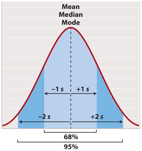
The normal distribution appears in countless applications in biology. Its shape is completely determined by two quantities. One is the mean, which tells you the location of the peak of the distribution along the x-axis (Figure 2). While we do not know the mean of the population as a whole, we do know the mean of the sample, which is equal to the arithmetic average of all the measurements—the value of all of the measurements added together and divided by the number of measurements.

In symbols, suppose we sample n individuals and let xi be the value of the ith measurement, where i can take on the values 1, 2, ..., n. Then the mean of the sample (often symbolized ) is given by , where the symbol means “sum” and means x1 + x2 + ... + xn.

For a normal distribution, the mean coincides with another quantity called the median. The median is the value along the x-axis that divides the distribution exactly in two—half the measurements are smaller than the median, and half are larger than the median. The mean of a normal distribution coincides with yet another quantity called the mode. The mode is the value most frequently observed among all the measurements.

The second quantity that characterizes a normal distribution is its standard deviation (“s” in Figure 2), which measures the extent to which most of the measurements are clustered near the mean. A smaller standard deviation means a tighter clustering of the measurements around the mean. The true standard deviation of the entire population is unknown, but we can estimate it from the sample as

What this complicated-looking formula means is that we calculate the difference between each individual measurement and the mean, square the difference, add these squares across the entire sample, divide by n - 1, and take the square root of the result. The division by n - 1 (rather than n) may seem mysterious; however, it has the intuitive explanation that it prevents anyone from trying to estimate a standard deviation based on a single measurement (because in that case n - 1 = 0).

In a normal distribution, approximately 68% of the observations lie within one standard deviation on either side of the mean (Figure 2, light blue), and approximately 95% of the observations lie within two standard deviations on either side of the mean (Figure 2, light and darker blue together). You may recall political polls of likely voters that refer to the margin of error; this is the term that pollsters use for two times the standard deviation. It is the margin within which the pollster can state with 95% confidence the true percentage of likely voters favoring each candidate at the time the poll was conducted.

Figure 3

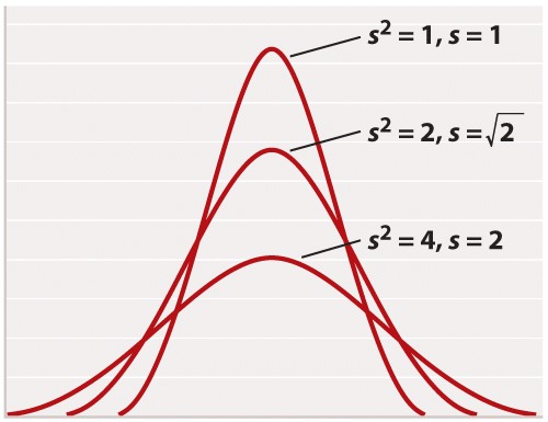
For reasons rooted in the history of statistics, the standard deviation is often stated in terms of s2 rather than s. The square of the standard deviation is called the variance of the distribution. Both the standard deviation and the variance are measures of how closely most data points are clustered around the mean. Not only is the standard deviation more easily interpreted than the variance (Figure 2), but also it is more intuitive in that standard deviation is expressed in the same units as the mean (for example, in the case of height, inches), whereas the variance is expressed in the square of the units (for example, inches2). On the other hand, the variance is the measure of dispersal around the mean that more often arises in statistical theory and the derivation of formulas. Figure 3 shows how increasing variance of a normal distribution corresponds to greater variation of individual values from the mean. Since all of the distributions in Figure 3 are normal, 68% of the values lie within one standard deviation of the mean, and 95% within two standard deviations of the mean.

Another measure of how much the numerical values in a sample are scattered is the range. As its name implies, the range is the difference between the largest and the smallest values in the sample. The range is a less widely used measure of scatter than the standard deviation.

Question

7qnN14FhO+DUltbUShQTDIQD65BLYQ1/jJaaMSwhf6cH0UdGOjXnBIGmP1pYtq+1RaV/AZU/1i3FXRVzxLpUqiVhz2I3AuLGca4b3zlE4Gneh2O7R1nVRR3uuK1TLRuvU1ExZGM91+vy3CTohenxU+7xvVc84/KSHeJbDjwysJ1J0Xy98ywGhG3/uqLGU/SpHjKtWoJsKP6btVFNAQKYPd6Cv6Er86xcUGVCty5eliDvhQ3DkKuDp71LkXGjZohzYWmNSZ8A8W7PYX25wnIRLDqVaxi68vYk/ikZaiKbqjAYpfaa6AL8lE1Dbuvj+AIERBCdZDgxco08he0Bl0WdUeDYT8pzJYilWR0n3g==
Correct.
Incorrect.
Incorrect. Please try again.
1

Question

KUHPMS6tkSAlANl30cBn2oWlPO02cDayO2wTg4qumg8l2f6EOQPPslday/eE0MmPl3MkM7XE1rPq7KeeT5iVvjfbz5qNN0986x/ts/zc9+WNHsUB/fQtGA/KGBRRryC1/u7lTKlnHa7vVTX5phOXu+nF6cG70NVsjtnnOvGokBkyIkhC/yuPnizQ4mzmX7uoXAoQlWs7+OiZMyuak0T27gXSQk30ym/8ZjlCXu7mtAmzP6dPN2Qrc6F+5+NWxJPkBd96gn/NOI7osOndqjnfrkh3ggbNQ0LABpRsEvTcfT9GucCmZkhGRgqT3QM02wnJlqxvvosPpjAmm3XEKVaorcNzDZ067TeJ3QqEziMnAk0o3BrLFNu1hnFiAa7HqmbnSIYBQU4hQgB9OE4diJYyS/A0zyaHnmACGX0d8cTDn2frxxK4zGRp0iSVY/U9RVdjCbavIfZgH6oGOaOOWZnQzbyasj3qumtRbxZPBc0ugt8i3GiBclH1378AGFz1YWyTCxxicrYbKfRXYY8U/t0Juw==
Correct.
Incorrect.
Incorrect. Please try again.
1

covariance A statistical quantity representing the extent to which the values of x and y change together. For every pair of values (xi, yi), you multiply the difference between each value and its mean, add the products across all samples, and then divide by n - 1.
correlation coefficient (r) A measurement of the strength of association between two variables.
Table

Statistics

Correlation and Regression

Biologists often are also interested in the relation between two different measurements, such as height and weight or number of species on an island versus the size of the island. Such data are often depicted as a scatter plot (Figure 5), in which the magnitude of one variable is plotted along the x-axis and the other along the y-axis, each point representing one paired observation.

Figures 5a and 5b

Figure 5A is the sort of data that would correspond to fingerprint ridge count (the number of raised skin ridges lying between two reference points in each fingerprint). While the data show some scatter, the overall trend is evident. There is a very strong association between the average fingerprint ridge count of parents and that of their offspring. The strength of association between two variables can be measured by the correlation coefficient, which theoretically ranges between +1 and –1. A correlation coefficient of +1 means a perfect positive relation (as one variable increases, the other increases proportionally), and a correlation coefficient of –1 implies a perfect negative relation (as one variable increases, the other decreases proportionally). Correlation coefficients of +1 or –1 are rarely observed in real data. In the case of fingerprint ridge count, the correlation coefficient is 0.9, which implies that the average fingerprint ridge count of offspring is almost (but not quite) equal to that of the parents. For a complex trait, this is a remarkably strong correlation.

Figure 5B represents data that would correspond to adult height. The data exhibit greater scatter than in Figure 5A; however, there is still a fairly strong resemblance between parents and offspring. The correlation coefficient in this case is 0.5. This value means that, on average, the offspring height is approximately halfway between that of the average of the parents and the average of the population as a whole.

The illustrations in Figure 5A and 5B also emphasize one limitation of the correlation coefficient. The correlation coefficient measures the strength of a straight-line (linear) relation. A nonlinear relation (one curving upward or downward) between two variables could be quite strong, but the data might still show a weak correlation.

Each of the straight lines in Figure 5 is a regression line or, more precisely, a regression line of y on x. Each line depicts how, on average, the variable y changes as a function of the variable x across the whole set of data. The slope of the line tells you how many units y changes, on average, for a unit change in x. A slope of +1 implies that a one-unit change in x results in a one-unit change in y, and a slope of 0 implies that the value of x has no effect on the value of y. The slope of a straight line relating values of y to those of x is known as the regression coefficient.

Covariance

Both the correlation coefficient and the regression coefficient are related to a value called the covariance between the variables x and y. The covariance is a statistical quantity representing the extent to which the values of x and y change together. For a sample of n pairs of values (xi, yi), where i takes on the values 1, 2, ..., n, the covariance (cov) between x and y is estimated using the equation

This means that, for every pair of values (xi, yi), we multiply the difference between each value and its mean, add the products across all samples, and then divide by n – 1. Again, the n – 1 has the effect of emphasizing that one cannot estimate the covariance between two variables by examining a single (x, y) pair.

If the deviation of an x value from its mean tends to have the same sign (positive or negative) as the corresponding deviation of the y value from its mean, then the covariance between the variables is positive. And if the deviation of an x value from its mean tends to have the opposite sign from the corresponding deviation of the y value from its mean, then the covariance between the variables is negative.

The correlation coefficient (r) between two variables expresses the covariance in terms of the product of the standard deviations, namely

where sx and sy are the standard deviations of x and y. Dividing the covariance by the product of the standard deviations removes the units of measurement and limits the range of the correlation coefficient from -1 to +1.

On the other hand, the slope of the regression line of y on x is given by a quantity often symbolized as b, calculated from a sample as

In the special case when sx= sy = 1 (as they are in Figure 5), the correlation coefficient and the regression coefficient are identical and both equal cov(x, y).

Question

j3+1g6YIToxlNmVIX4lf1DeFWBIe51OazwwUYj58wwtHC6si37PALWRSdUKrjqj3SkQUUV+WKzfua66rwIHFE/XHni8Hq5GK20kPM2gwmobDEZFVEq6K0zHxiVfjOwu7lAVgqxp8DmPKlrUr6++gx49UdMmy+KZUt83jWjoXb9veS2u0hVS+++Ij/VCpEMrX3uUtw9qauyH7bM7pT+zfOvxelpd+9dKvSi0ZB4U/BSQEwsWPenkxIFYAvy6G9oJSOeZbcf8152tkutcvU9XoanasnUguzZ5m9i86BpBWxdeezubu0HYpLLK/NwG+iAll8KUSE45WjeiSad/Ny7NnqtM6uIev9Phf9J+Lcn6Av9eky5WzgmspgjLSqR5xocnwukeHMd5tPPzQE4ccysWX+5j2ROOxNdhKoGpw/EXX+VvK6vjQc2PqL8lgq9QTpkxfOdg6G1mO/pVFSQ5e20Ioxll9mX3cQrHUn4rxJiLmjc6OSed3UlyBnSXzIodi7vxijedMk7RXCAuUQCJH1QdEyAwoK5OeJg2mXIeRStntkqSkxgKQNIYwh1Rq/QSZeP5ei0A8eB0ttzH9HQIAn7KjoNIO+rCSHWQP5EiWMfacq6uSgITmJn7ArQ==
Correct.
Incorrect.
Incorrect. Please try again.
1

statistical test A test used to distinguish accidental or weak relations from real and strong ones.
P-value The likelihood that an observed result (or a result more extreme than that observed) could have been observed merely by chance. If P ≤ 0.05, the observed results are conventionally regarded as unlikely to be attributed to chance alone.
Table

Statistics

Statistical Significance

Biologists observe many relations between variables that are either due to chance in the sample that happened to be chosen or that are too weak to be biologically important. To distinguish the accidental or weak relations from the real and strong ones, a statistical test of the relation is carried out. A statistical test must be based on some specific hypothesis. For example, to determine whether an observed correlation coefficient could be due to chance, we might carry out a statistical test of the hypothesis that the true correlation coefficient is 0. A statistical test usually yields a single number, usually called the P-value (or sometimes p-value), that expresses the likelihood that an observed result (such as a correlation coefficient) could have been observed merely by chance. A P-value is a probability, and if P ≤ 0.05 the observed results are conventionally regarded as unlikely to be attributed to chance alone. In that case, the observed relation is likely to be genuine. In other words, if an observed relation would be obtained by chance alone in only 1 in 20 or fewer experiments (P ≤ 0.05), then the observed relation is regarded as likely to be true. A finding of P ≤ 0.01 is taken as even stronger evidence that the observed result is unlikely to be due to chance.

Figure 6

Statistical testing is necessary because different researchers may disagree on whether or not a finding supports a particular hypothesis or if the interpretation of a result could be affected by wishful thinking. Take Figure 6, for example. If you wish to believe that there was a functional relation between x and y, you might easily convince yourself that the 20 data points fit the straight line. But in fact the P value of the regression coefficient is about P = 0.25, which means that about 25% of the time you would get a line that fits the data as well or better than the line you observed, purely by chance. The proper conclusion is that these data give no support for the hypothesis of a functional relation between x and y. If there is such a relation, then it is too weak to show up in a sample of only 20 pairs of points.

There is good reason to be cautious even when a result is statistically significant. Bear in mind that 5% of statistical tests are misleading in that they indicate that some result is significant merely as a matter of chance. For example, over any short period of time, about 5% of companies listed in stock exchanges will have changes in the dollar value of their shares that are significantly correlated with changes in the number of sunspots, even though the correlation is certainly spurious and due to chance alone. Critical thinking therefore requires that one maintain some skepticism even when faced with statistically significant results published in peer-reviewed scientific journals. Scientific proof rarely hinges on the result of a single experiment, measurement, or observation. It is the accumulation of evidence from many independent sources, all pointing in the same direction, that lends increasing credence to a scientific hypothesis until eventually it becomes a theory.

Question

JC1WSVCkvJJADSSItEMe6pkiF46n8zSaADdu7pQmnmYS+zjEN3G8nUj6xPxvdLa/9mjIAfPs2/8VaUVpqsOB2udHR8/iSoDmhoU9JF7DTI3A/YrKIudESMCC4E/8g8sb2iQ/xf1daz2GqR/ELT3PDcTK9X9oCDBv5ENzmijMkvNclRtgt6fNsJF6OlAPQWB38t7OfgVRuRXnZJQc3XWat5HsCgE8PipTLXop489F++b1PwoBuVP4/ZdUEm3+THatgSCo4+hlxgXjmOCegg2MFo9xksDbTHZyV5qIf7FQIlpPqnFnyogxNCqEgl9w+l95JO85FHshTIRfb4KqU5Z+byo5S4LBTGZpB8q3yWz7+JvVI1Z8ORaiZYbpPETlHp277OwA0F7gHwy6s430thqkHIqywslgCjrK/nbzZO5EenVx5wGYxpLcCT2VhWtqs7LG6MnM6+tCz6v5INI+BHgv/+KdmpL622utVwO/rj/JlLsrM7BJJ2j+hvNXj80GjUugPFsv5A+mVHa9B0MBy77+UQRgIKvyUELCNVbg1MZGMeHiR2BP80MiuVYDSAs1Zjd21+sk7dVTBXlm62Xqbedzp3JsGvwROiZqoRhxnmiK+NnJ2q3czRllRbvK47FwPS9eFWYT1bi91ijXLCDU2sgFYpnYbnQh7hUnRE9I+CzhUYBHZgAxFdlWe9oTXeuGajN3efZ7qkbs6d7UmAoA1unb5p8bhhmP3bZkFEdxE3qKM0pQwiltBIu+ylNBJOWU5SZC5UrzTQ==
Correct.
Incorrect.
Incorrect. Please try again.
1

positive correlation An association between variables such that as one variable increases, the other increases.
Table

Statistics

Correlation and Regression

Biologists often are also interested in the relation between two different measurements, such as height and weight or number of species on an island versus the size of the island. Such data are often depicted as a scatter plot (Figure 5), in which the magnitude of one variable is plotted along the x-axis and the other along the y-axis, each point representing one paired observation.

Figures 5a and 5b

Figure 5A is the sort of data that would correspond to fingerprint ridge count (the number of raised skin ridges lying between two reference points in each fingerprint). While the data show some scatter, the overall trend is evident. There is a very strong association between the average fingerprint ridge count of parents and that of their offspring. The strength of association between two variables can be measured by the correlation coefficient, which theoretically ranges between +1 and –1. A correlation coefficient of +1 means a perfect positive relation (as one variable increases, the other increases proportionally), and a correlation coefficient of –1 implies a perfect negative relation (as one variable increases, the other decreases proportionally). Correlation coefficients of +1 or –1 are rarely observed in real data. In the case of fingerprint ridge count, the correlation coefficient is 0.9, which implies that the average fingerprint ridge count of offspring is almost (but not quite) equal to that of the parents. For a complex trait, this is a remarkably strong correlation.

Figure 5B represents data that would correspond to adult height. The data exhibit greater scatter than in Figure 5A; however, there is still a fairly strong resemblance between parents and offspring. The correlation coefficient in this case is 0.5. This value means that, on average, the offspring height is approximately halfway between that of the average of the parents and the average of the population as a whole.

The illustrations in Figure 5A and 5B also emphasize one limitation of the correlation coefficient. The correlation coefficient measures the strength of a straight-line (linear) relation. A nonlinear relation (one curving upward or downward) between two variables could be quite strong, but the data might still show a weak correlation.

Each of the straight lines in Figure 5 is a regression line or, more precisely, a regression line of y on x. Each line depicts how, on average, the variable y changes as a function of the variable x across the whole set of data. The slope of the line tells you how many units y changes, on average, for a unit change in x. A slope of +1 implies that a one-unit change in x results in a one-unit change in y, and a slope of 0 implies that the value of x has no effect on the value of y. The slope of a straight line relating values of y to those of x is known as the regression coefficient.

Question

8ZJ2sh071VhniFwE4gs7nTsa4nTWXnLsBRGimuQ0nQb/P8VOGPdLgj5w8CnHJLerVqHRPla4bqe4hGbPGkpqqFusCu6b/1KEGHKOTaCEkSHWi77kvRnTz/GImVGK/mpx8eggiuMC1A2PUmhzNysEjLOD90kiG+ZM0Nq7NAUxgjFkKCZpw6bmQcCsOabYRjneXQ/udkASorRZ+neDVoopVXhWNCVqF/+zT8q1QT6hd/FsemGXRg7GfIzPtRWspB3oSB4cpd9hT0Kd8KaUDpoUIT8xNK1U/sMHimsiBHMArHQ+P4EAYvo4WN3E5+MMCA19VcPHZQKHhcmqr7I/QG7aSCDFb+JAPYGh4nTTm7AN/6r/p/FT
Correct.
Incorrect.
Incorrect. Please try again.
1

Question

eu+110maomxi+HDd31o0ipzBdjjolk24X0kiYti5v8tJSMGD+b0+YpPsiZFc9dOby2N0ghliPrM9UPOc4MiDFrxKSIjh4W/eJwlWs/KoHb+6P3E6F66p4kUX+3KGAosW55W+6m4AX6BIgk6YibtH6tkQoP8HvniatvD2luXGA9JuxSDDY4dFnSkPYoQVS6dHoWknIlD9mlnVwaf+xSNsceNAefqUsRSlC846L2HHmBnMBY8T8iENhkccm6CvjTaJAbnoQjyzbJ91ciNbgtVMDyXMtWhDjFqhr3NOTLhNERUBG1sJjp7s8Ql6L2k0JZ1h96qHqwfM4HTniWoQ+ROy07XwyCR/dpTaRp4hOa3FpH+jJlAOoEPaZmg0mQvxtc0O7z8CN04sQDj2Ed5KT6BoyXfD2w/i8LIJLMcbNCJYOQFrSHiGma2oQ40uZhJKUPWmkCoiDWmePuuxatZQCrHZzR9xJ7QhjuRRdyezgzVU6/a4799T95ZRiIdbmHOguNOvDjJqwQ==
Correct.
Incorrect.
Incorrect. Please try again.
1

Question

ThLlNMfFjRcnp2hSBsb+ZE9ebdf9fOu3eI1vv6lXuRVdnbj440DO7cN4+1KOnNP3R2qa2yPvKBYTkTl3rIuFwXQC6QiulxX1er+xb/0HJmqYCHHNCSPARe/BUXqYqH6XE7fQgk0prKL4EnbJX+QNp1hwtve7Cpuieuz7asPOx4nhAVk4QamwmgIUN7bTYiqosIVtowZZFKj0LZLus7uE53wc/pM19EVGutZqWl5rnhcMVtuGiz4lqsYCTMB+avASSawVhnlG4wWbnSJMB3A5PvleE5HY+r+LtbbMXLvKOUAIsI+os3EP3Ctytp266b8N+pd9U2KAvuRkQKK8W3Sh61jW9e5Si/pGYP/TzybWy1eEhwziocTL6OegIIey0OOfmVLePDsf5ob2XwYjp9FkHQ/TocCTQoojD4Hur9xpsBH6fABPnmXxhEz5eb9hkt94RVmfs0X2hR1yjg3s+dSW8c6fdPBBKvHbBzsYWcJBxysYjNcRsdiu6R5C0vv25p9WQLJzrYtQfIFkmLt24rJoke+vRTpC0XxPp61vrxUaesbD5/tjwf4j+URYHKaX06sdEbQb9FPsYHY=
Correct.
Incorrect.
Incorrect. Please try again.
1

Question

/nlnxshmI61YuDhsnTo1IiVbv3rzErYOvTv13jfPG8XGwFSiN8KcDKx5dngfV+5CrLSNw775ozrqk4zkRH9EbiXYZQm9POgE3a3KChrNJU4/TIrqR0F/frUA+4Hcys2FbsrMMyAxA+qshBQ05dd9sQPNLOS5d3OT1WOKsrjlR87yN0/kegg7Y65s3o5p8G3ifd9faIpf83jNU85sVbD0v6cVJh2RSzKFi9KOvzjgSiRbfTw7kuAg1HlVjhxuLZwNtmwCEEZBKcdm+QVypg2M/1VqJOmY56s0/E1Wd9VhTneqv/SxyqCvbJyfckqcNHgbK6eGUW/Tl3mIOz9n5tk8ujHbK1Mp92x7Cnjmt4dEx/T2fmZtw1AfkHHNVh0OYsYQvIx+DSc5SQPujvfGqz+nNAQMfIW12Hb0dD3Obc0VjRl3GE6MkRuAwXK9DHfAsbSMU5HTVSKNf5LyM4fzj5A80KqlBRoQMlnY9yk/Nt3yhRW28SHmasuoptJwDK223J0gmZspCWEgkip9+4VF3qX865giBhGXzWKQV5pMxeY34/qX4QfTthxauchr3Rp3nHSS1zfVgGOKvl+hPGZ6uBTDvhTiZnCDJXfNM8JYj4pE5JXThqiCwD8IKidnZvU=
Correct.
Incorrect.
Incorrect. Please try again.
1

Question

BwVMNu0hrVMrGS9NwUhSUANLje1EotEl/r8Htrhvkomgh9VpvyTDwN3PidNRBcLBgFmZLddgOppTCfI/8Jtdmc8i4kMFJueUqb00P3aKmP0yLsDsfi6rCapla77uj6aEJYmCrWdGhB48/tmcL8o0dV2LnmLUNEw23FeymVUQmGIOK9U5wHXJvgq9gWrPGmIh9pKo89ICmkW70SLh7Y7nY+wXI7rgF/ob1SiVREWXUMQEvXpJbGB8LJZXlZqvAzbQovjOvz7nZkvct4PQ6prMsuWRjY/nWTd6qNo7iGk3WuLeP6EMBBwOyKX1z4wZxYsgiYHynSlWSgB9lVsD8G78CVVqQ6oq3lanVro+j7EVnOjrZEdy4ZdLngq9gebnxzpun/oggAIXNAnmHrB0n4LBTnG+NK9A+A0+w7AM/fv9z1UBLfp+uwVulsCJL/1mL7ZWeEs+ZQgHQrD5u0b0hl00gvuMxmwRcoyaLGTGnUYwTID2crK2lRTJejCxFVJKg0evjBmVEzJw73go5zYsYSBRx2yPzBIRqtXoAtDdN3KO+tlmetKsZTjiJY38NTWNSBLJCoPdgjNWHLW0tDtLZPwqM67BoZ34Y++S
Correct.
Incorrect.
Incorrect. Please try again.
1

Question

N83z5YxM7np93xwr8qumyxj92iEWpShEC+mmm6+qoLqbJ5NaxyKHJmuHeDBdxIz05WjMBTuBwoT2MTvdxT9sRBcbVGDL9uDzsefTEbLPY8DGfGjzGIHUYqA4anTV/hCZxrZ/ZGBSbMHiKAm+Z9SaaCn0XzOrS6inVDRBFA/DFgor+eYmB6Jr8djsIOCgDxtt3+PYNiMVWH3+JdkJruzxwy3NmqkF7uhCLmAnsEcCRF01HaK6Y6X8L2ddck2w2QFvhZ5TjsgpO6Hg5J5PFkKUE+9v/Bi4ZhlpLfbVVjN8I6SHMcayDwGdXGfe87ggpkIsDpyZg1MvohnQwDySU+iV7kJLZK9mkyyCbwQGd27LiZzx8setCztynRWZeUhDwvutfkGbqolg+KTXCwAtIus6/lKTWuhJuutuvj+xAaPlBT+iOvZdyE+5Gf1Y55DA9abx8XzCbJ4bq3+73/9F6dnN2zgfUPIBssHUh4wctiFLBeOf7ZIK4PYI7E1a/lYE1UK0r8odWZLq+a0bnThN
Correct.
Incorrect.
Incorrect. Please try again.
1

Question

jpjjQ39WxppkrNZAIzfhiX2020bItiAge54SF8I8Tk0BJqcOUCaq6GZegGCgCluWi+q1/HMxdv/YYAJmh1n4K5LXVDXEoW/ZMfbG6hTM89FVgzLp5OjsikIaAKSi6yD0Wgfwms+6HQb9Hr4Fl4kM+9FzQihZ43EQHhAsPvJVTXOecsTOEO3Tm4CWV3EpbMmBcNh5ix763JgPi2rt+1DcfI4gcXuvaMlcuDrQ8ETSyQqeJzmolxQXdbXZ6CGfEvBZDMVBsxIiHeiMOHuNZcYj6D++Scl4enVy9e4b7OkLLOBN4y7x6Pl7tB/lCs/LkCHXv/dn3Q==
Correct.
Incorrect.
Incorrect. Please try again.
1