Chapter 1. Working With Data 29.11
Working with Data: HOW DO WE KNOW? Fig. 29.11
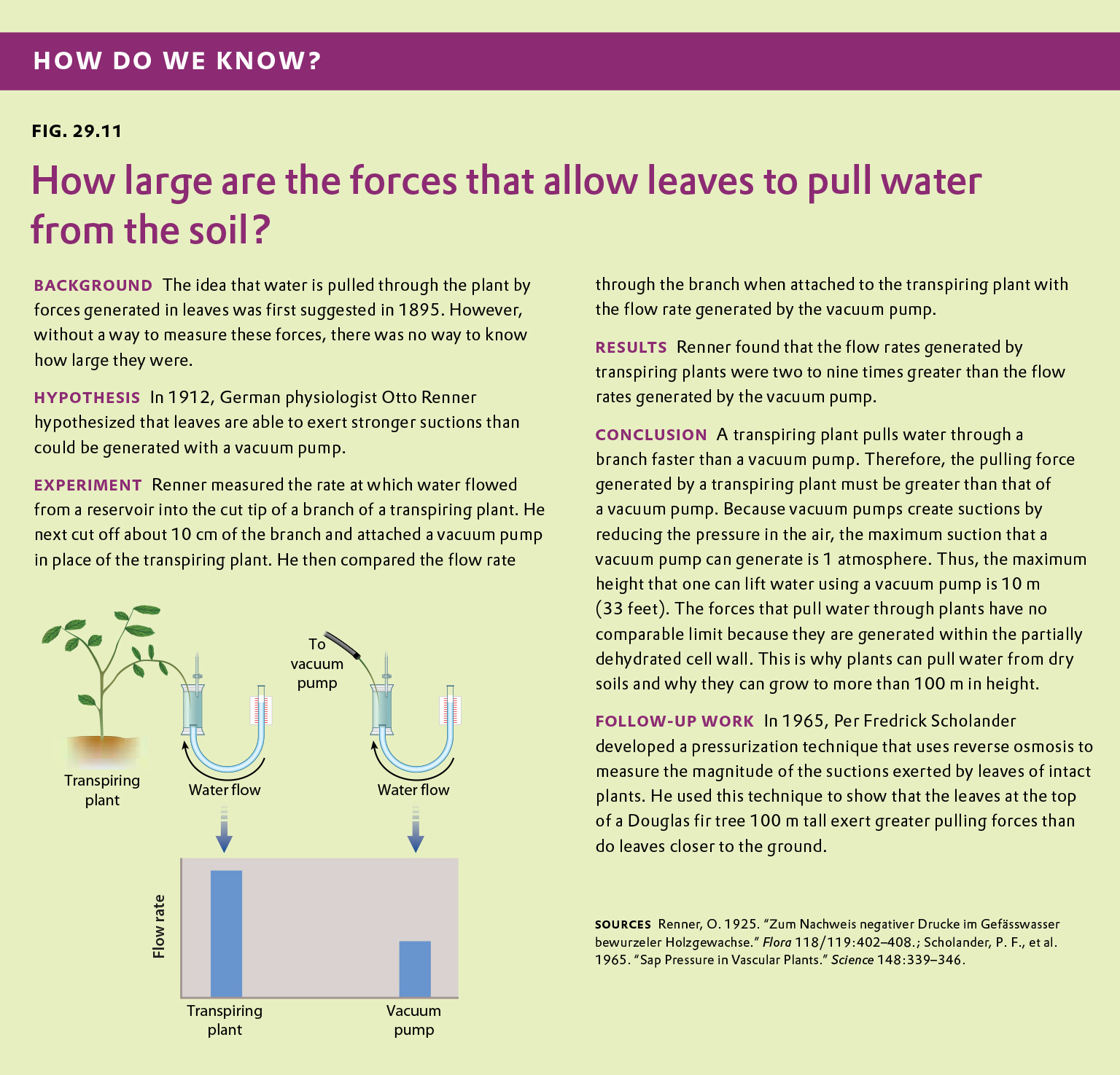
Fig. 29.11 describes Otto Renner’s experiment showing that leaves exert stronger forces on water being pulled from the soil than a vacuum pump could. Answer the questions after the figure to practice interpreting data and understanding experimental design. These questions refer to concepts that are explained in the following three brief data analysis primers from a set of four available on LaunchPad:
- Experimental Design
- Data and Data Presentation
- Statistics
You can find these primers by clicking on “Experiments and Data Analysis” in your LaunchPad menu. Within the following questions, click on “Primer Section” to read the relevant section from these primers. Click on the button labeled “Key Terms” to see pop-up definitions of boldfaced terms.
Question
In the original paper published by Otto Renner, all of the flow rates measured into intact plants were greater than what could be produced by a vacuum pump pulling water through the same branch segment. Under what conditions would you predict that Renner would have measured a lower flow rate into the intact plant than subsequently measured using the vacuum pump?
| A. |
| B. |
| C. |
| D. |
Question
In your work as a plant physiologist, you encounter a population of plants with a mutation that causes their xylem vessels to be only half the diameter of the xylem vessels produced by plants that do not have this mutation. You hypothesize that the plants with the smaller-diameter xylem vessels generate greater pulling forces (compared with the wild-type plants) in order to supply their leaves with water. To test your hypothesis, you make the same measurements as Renner did to determine the pulling force exerted by the mutant (Pmutant) and the wild-type (Pwildtype) plants. What is your null hypothesis?
| A. |
| B. |
| C. |
| D. |
| null hypothesis | A hypothesis that is to be tested, often one that predicts no effect. |
Experimental Design
Types of hypotheses
A hypothesis, as we saw in Chapter 1, is a tentative answer to the question, an expectation of what the results might be. This might at first seem counterintuitive. Science, after all, is supposed to be unbiased, so why should you expect any particular result at all? The answer is that it helps to organize the experimental setup and interpretation of the data.
Let’s consider a simple example. We design a new medicine and hypothesize that it can be used to treat headaches. This hypothesis is not just a hunch—it is based on previous observations or experiments. For example, we might observe that the chemical structure of the medicine is similar to other drugs that we already know are used to treat headaches. If we went into the experiment with no expectation at all, it would be unclear what to measure.
A hypothesis is considered tentative because we don’t know what the answer is. The answer has to wait until we conduct the experiment and look at the data. When an experiment predicts a specific effect, as in the case of the new medicine, it is typical to also state a null hypothesis, which predicts no effect. Hypotheses are never proven, but it is possible based on statistical analysis to reject a hypothesis. When a null hypothesis is rejected, the hypothesis gains support.
Sometimes, we formulate several alternative hypotheses to answer a single question. This may be the case when researchers consider different explanations of their data. Let’s say for example that we discover a protein that represses the expression of a gene. Our question might be: How does the protein repress the expression of the gene? In this case, we might come up with several models—the protein might block transcription, it might block translation, or it might interfere with the function of the protein product of the gene. Each of these models is an alternative hypothesis, one or more of which might be correct.
Question
After making the measurements, you organize your raw data into a data table, shown below. In this table, Flowplant is the flow rate into the intact plant and Flowpump is the flow rate through the branch into the vacuum pump.
| Population A | |||||
|---|---|---|---|---|---|
| Plant 1 | Plant 2 | Plant 3 | Plant 4 | Plant 5 | |
| Flowplant (μg/min) | 6.3 | 5.7 | 3.8 | 3.2 | 9.7 |
| Flowpump (μg/min) | 0.3 | 0.29 | 0.17 | 0.15 | 0.51 |
| Population B | |||||
| Plant 1 | Plant 2 | Plant 3 | Plant 4 | Plant 5 | |
| Flowplant (μg/min) | 52.3 | 22.8 | 18.2 | 36.7 | 15.0 |
| Flowpump (μg/min) | 4.9 | 2.3 | 1.7 | 3.8 | 1.5 |
In order for these data to be consistent with your hypothesis, which population (A or B) is made up of the mutant plants and which population is made up of the wild-type plants?
| A. |
| B. |
| raw data | A series of observations or measurements. |
| data table | A table presenting data, typically categorized in some way. |
Data and Data Presentation
Processing Data
Initially, we have raw data—our series of observations or measurements. Before we move to the next level of data analysis and presentation, we often need to process the raw data in some way. Sometimes, for example, this may entail transforming a long string of numbers into a data table. To do this, we may need to categorize the data. For example, in our forest example, imagine that over a 24-hour period in our forest patch, we count 108 sightings of mammals. The first step is to categorize the sightings according to species and put the data in table form. In this case, we generate a frequency table in which we specify the number of sightings of each of six mammal species, A–F:
| Species | A | B | C | D | E | F |
| Number of sightings | 43 | 47 | 3 | 5 | 7 | 3 |
This table illustrates the pitfalls of data collection and how we have to be very careful when we design our data collection protocol. How valid are these data? We have seen B’s many times, but maybe each sighting is of the same individual. It is possible that all 47 B sightings were the same individual, whereas perhaps the three F sightings were three different individuals. This suggests that the design of our sampling scheme was flawed. We should re-do the census, only this time using traps that can mark each individual. Imagine that the revised method results in the following numbers:
| Species | A | B | C | D | E | F |
| Number trapped | 17 | 29 | 5 | 2 | 5 | 3 |
Question
You now conduct a statistical test to determine whether the mean value of the pulling force measured for population A (¯xA) is equal to the mean value of the pulling force measured for population B (¯xB). It may seem strange that we are testing the null hypothesis (¯xA = ¯xB) rather than our hypothesis (¯xA ≠ ¯xB).
However, as stated in the Experimental Design primer: “Hypotheses are never proven, but it is possible based on statistical analysis to reject a hypothesis.” If there is a low probability that the null hypothesis is correct, we can “reject” the null hypothesis with a level of confidence described by our statistical test, and thereby gain support for our alternative hypothesis.
The P-value for the statistical test is: P < .01. This means that:
| A. |
| B. |
| statistical test | A test used to distinguish accidental or weak relations from real and strong ones. |
| P-value | The likelihood that an observed result (or a result more extreme than that observed) could have been observed merely by chance. If P ≤ .05, the observed results are conventionally regarded as unlikely to be attributed to chance alone. |
Statistics
Statistical Significance
Biologists observe many relations between variables that are either due to chance in the sample that happened to be chosen or that are too weak to be biologically important. To distinguish the accidental or weak relations from the real and strong ones, a statistical test of the relation is carried out. A statistical test must be based on some specific hypothesis. For example, to determine whether an observed correlation coefficient could be due to chance, we might carry out a statistical test of the hypothesis that the true correlation coefficient is 0. A statistical test usually yields a single number, usually called the P-value (or sometimes p-value), that expresses the likelihood that an observed result (such as a correlation coefficient) could have been observed merely by chance. A P-value is a probability, and if P ≤ 0.05 the observed results are conventionally regarded as unlikely to be attributed to chance alone. In that case, the observed relation is likely to be genuine. In other words, if an observed relation would be obtained by chance alone in only 1 in 20 or fewer experiments (P ≤ 0.05), then the observed relation is regarded as likely to be true. A finding of P ≤ 0.01 is taken as even stronger evidence that the observed result is unlikely to be due to chance.
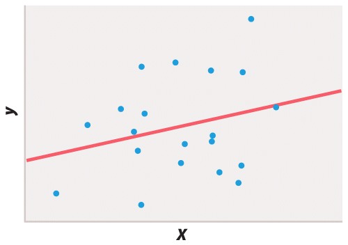
Statistical testing is necessary because different researchers may disagree on whether or not a finding supports a particular hypothesis or if the interpretation of a result could be affected by wishful thinking. Take Figure 6, for example. If you wish to believe that there was a functional relation between xand y, you might easily convince yourself that the 20 data points fit the straight line. But in fact the P value of the regression coefficient is about P = 0.25, which means that about 25% of the time you would get a line that fits the data as well or better than the line you observed, purely by chance. The proper conclusion is that these data give no support for the hypothesis of a functional relation between x and y. If there is such a relation, then it is too weak to show up in a sample of only 20 pairs of points.
There is good reason to be cautious even when a result is statistically significant. Bear in mind that 5% of statistical tests are misleading in that they indicate that some result is significant merely as a matter of chance. For example, over any short period of time, about 5% of companies listed in stock exchanges will have changes in the dollar value of their shares that are significantly correlated with changes in the number of sunspots, even though the correlation is certainly spurious and due to chance alone. Critical thinking therefore requires that one maintain some skepticism even when faced with statistically significant results published in peer-reviewed scientific journals. Scientific proof rarely hinges on the result of a single experiment, measurement, or observation. It is the accumulation of evidence from many independent sources, all pointing in the same direction, that lends increasing credence to a scientific hypothesis until eventually it becomes a theory.
Question
Your hypothesis that the plants with the smaller-diameter xylem vessels generate greater pulling forces (compared to the wild-type plants) is based on the fact that it is harder to push (or pull) water through a narrow tube than through a wider one. In fact, as described in Chapter 29 (p. 608), the flow rate through a xylem conduit (or any tube) is proportional to its radius raised to the fourth power (assuming the force pushing or pulling the liquid through the tube is held constant). If the pulling forces generated by the leaves of the mutant and the wild-type plants were equal, what would you expect the flow rate through the xylem of the mutant plants to be compared to the flow rate through the wild-type plants?
| A. |
| B. |
| C. |
| D. |
| E. |
Question
Your data, however, shows that the mutant plants generate greater pulling forces compared to the wild-type plants. Based on your data in the table shown in question 3, as well as the 2-fold difference in conduit width, what would you expect the flow rate through the xylem of the mutant plants to be compared to the flow rate through the wild-type plants?
| A. |
| B. |
| C. |
| D. |
| E. |
| F. |
| G. |
| H. |
| I. |
Question
One detail of the Renner experiment that was not mentioned in Fig. 29.11 was that Renner applied a strong clamp around or cut multiple grooves into the branch before making his measurements. The presence of the clamp or the grooves created a “locally defined resistance” that reduced the rate at which water flowed into the plant and into the vacuum pump. Why did Renner add this resistance?
| A. |
| B. |
| C. |
| D. |
Question
You now set out to investigate the effects of gravity on water in the xylem using the Renner method. You decide to make your measurements at night. Your reasoning is that when the stomata are closed there will be no flow of water through the xylem and thus any pulling forces within the xylem should reflect what is needed to hold the water column upright against the force of gravity. You hypothesize that the pulling force measured at night will increase with height above the ground at which the measurement is made.
The following graphs show the measured flow rates plotted as a function of the height of the branch.
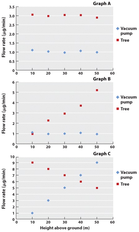
Which of these graphs is consistent with your hypothesis?
| A. |
| B. |
| C. |
Question
Which of the graphs in question 8 is consistent with the null hypothesis that the pulling force measured at night is independent of height?
| A. |
| B. |
| C. |
Question
A vacuum pump is able to pull water up to a height of 10 meters (33 ft). If you were to measure the flow rate through a branch connected to the tree at 10 m above the ground (at night and with wet soil), what would you expect the flow rate to be relative to the flow through the same branch when measured using the vacuum pump?
| A. |
| B. |
| C. |
| D. |
Question
You return to the same plant after two weeks without rain (so the soil was dry) because you are interested in how the dry soil affects the pulling forces within the xylem. Under these conditions, what would you expect the flow rate to be into the intact branch at 10 meters above the ground (relative to the flow through the same branch when measured using the vacuum pump)?
| A. |
| B. |
| C. |
| D. |