Chapter 1. Working With Data 7.12

Working with Data: HOW DO WE KNOW? Fig. 7.12

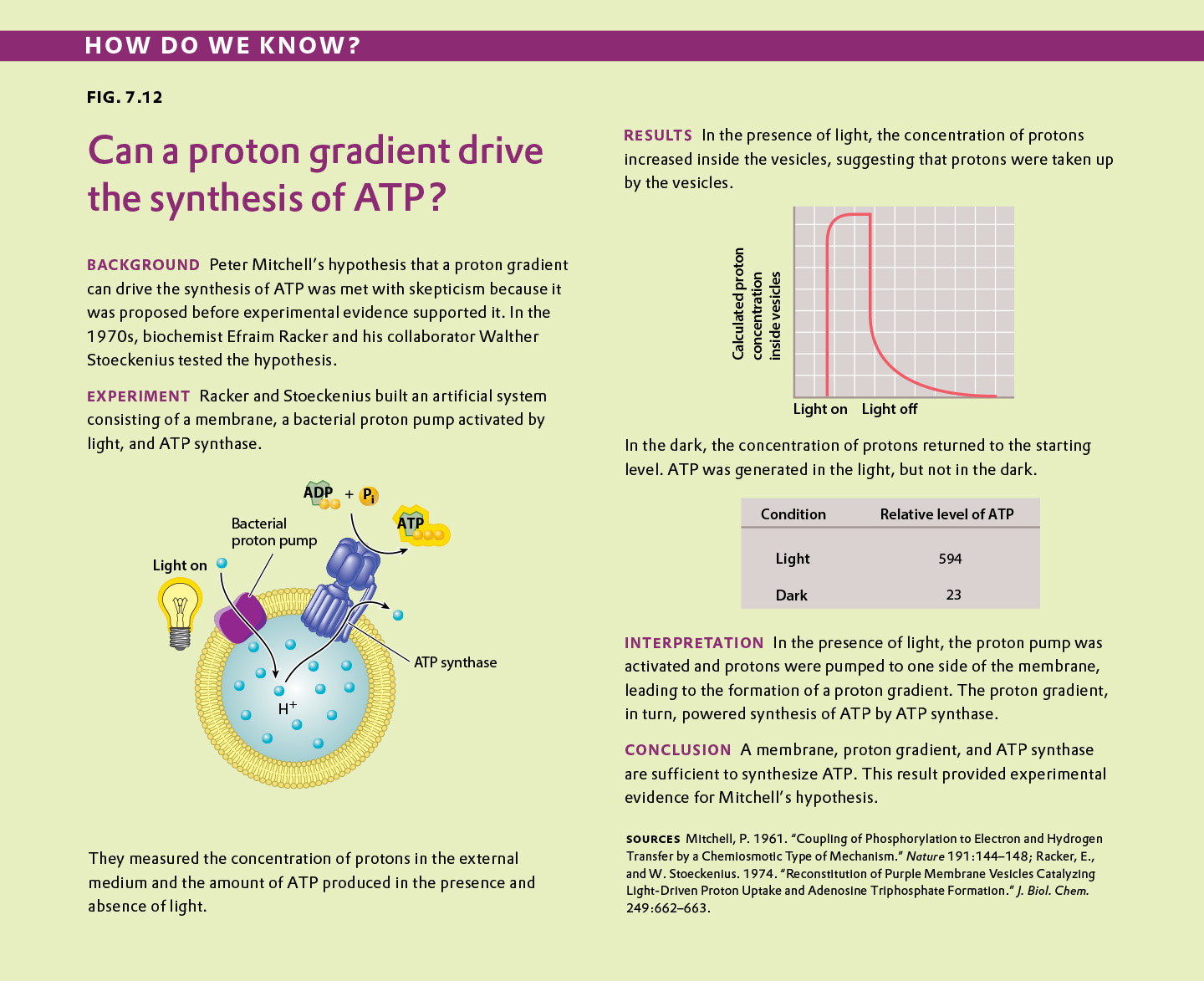
Fig. 7.12 describes experiments linking a proton gradient to the synthesis of ATP. Answer the questions after the figure to give you practice in interpreting data and understanding experimental design. Some of the questions refer to concepts that are explained in the following three brief data analysis primers from a set of four available on Launchpad:

  • Experimental Design
  • Statistics
  • Scale and Approximation

You can find these primers by clicking on “Experiments and Data Analysis” in your LaunchPad menu. Click on “Primer Section” to read the relevant section from these primers. Click on “Key Terms” to see pop-up definitions.

Question

QNzmtMnwuD1wC7rN9P01Mmuxbcu0FGblXCYyhlaUlKQxubAxnaS+FZwtWUimzZ+DDgvFyKbYvDBl39GV00cy1zvfoT2rEJmv+clLSjDnf8cVrxGQMETov0gmOI/tEWEXwo/oXVnnhqXqJfBqQjrg8aoBomuHxaLRj3lX9Rh3vH+kMxBb9QJtg4BNSueSlugppXbR95xOz4djpqlLCldifB9GZTsJU6Lk9SkyGR9eQMPK30Eg0hnuAkkkvF7lpIZhP3eKca7/HaQAqzlITtlJ7iHkuKL8X0EdXIQqjL2radVBz724Zx4krXvDyRa/GDfnExE+I1OipSAEAmK/6xVN+rhZKnAirkTmCVVyVW7JH9SDOY+dv0llvGdq6TJUJ4RXQbxS/skUYiLIqxm+493VDVkalsJVh+ZN4Vm0vt5JnonAqZxwo93w5ritqJ0N1LmBnaAIbpB6BhYAZT6YW2Q0Tp1Q2fspmsToSCy3A9iqrjJxZqEMu77rJpa/jWSdQG49QvPjzHqcm+U5JBg5dsBOO4uRD/Ii+jyKXt6ZX1YlLEA2QF8FObNLaymCHKQazFiKWnTJXA==
Correct.
Incorrect.
Incorrect. Please try again.
1

hypothesis A tentative explanation for one or more observations that makes predictions that can be tested by experiments or additional observations.
Table

Experimental Design

Types of Hypotheses

A hypothesis, as we saw in Chapter 1, is a tentative answer to the question, an expectation of what the results might be. This might at first seem counterintuitive. Science, after all, is supposed to be unbiased, so why should you expect any particular result at all? The answer is that it helps to organize the experimental setup and interpretation of the data.

Let’s consider a simple example. We design a new medicine and hypothesize that it can be used to treat headaches. This hypothesis is not just a hunch—it is based on previous observations or experiments. For example, we might observe that the chemical structure of the medicine is similar to other drugs that we already know are used to treat headaches. If we went into the experiment with no expectation at all, it would be unclear what to measure.

A hypothesis is considered tentative because we don’t know what the answer is. The answer has to wait until we conduct the experiment and look at the data. When an experiment predicts a specific effect, as in the case of the new medicine, it is typical to also state a null hypothesis, which predicts no effect. Hypotheses are never proven, but it is possible based on statistical analysis to reject a hypothesis. When a null hypothesis is rejected, the hypothesis gains support.

Sometimes, we formulate several alternative hypotheses to answer a single question. This may be the case when researchers consider different explanations of their data. Let’s say for example that we discover a protein that represses the expression of a gene. Our question might be: How does the protein repress the expression of the gene? In this case, we might come up with several models—the protein might block transcription, it might block translation, or it might interfere with the function of the protein product of the gene. Each of these models is an alternative hypothesis, one or more of which might be correct.

Question

Yr6SDZGFvq8ijMe8vZhFhIXof0W6cqkP1iR4X4pSny/f+jXre6NvE5g1HE646SVK3vxOaV/DWHUWWzZmZ/9f+2hDpq4IK4pAwW3t3XJXHYV/M1LTXoPqE1JXAamk53evsOIlXnY9h2zyH7/Jw672La2PKjLPy9bGmWvrzrcT082pWu1Cm5jYEoK94wmhXiiyUmVEJDZ5/0SoCgPtjF0iTy42mMO7jSL9lNmR2Dg4ywhBvv4WDxYIkf98Vk7W4JeWJ1j14EvYA1IspPvQzo/Zjc/Oe8r/2ibLkD6w2s1CxaZWkZFga6NwNTh5VXKePG6gUQ3bqSpXXI75l0V0KH5durdfEMKtE4Bj8iDSR89JGtokYVz8NwoILPmkVoB8/oyz8vIKeRMEQPV1aq7WUWU4p98vLrVUPuuk32lDvUrJutfQ07arP5+Phw==
Correct.
Incorrect.
Incorrect. Please try again.
1

dependent variable The effect that is being measured.
Table

Experimental Design

Testing Hypotheses: Variables

When performing experiments, researchers manipulate the test group differently from the control groups. This difference is known as a variable. There are two types of variables. An independent variable is the manipulation performed on the test group by the researchers. It is considered “independent” because the researchers could choose any variable they wish. The dependent variable is the effect that is being measured. It is considered “dependent” because the expectation is that it depends on the variable that was changed. In our example of the headache medicine, the independent variable is the type of medicine (new medicine, no medicine, placebo, or medicine known to be effective). The dependent variable is the presence or absence of headache following treatment.

In designing experiments, there is an additional issue to consider: the size of each of our groups. In order to draw conclusions from our data, we need to make sure that our results are valid and reproducible, and not merely the result of chance. One way to minimize the effect of chance is to include a large number of patients in each group. How many? The sample size is the number of independent data points and is determined based on probability and statistics, the subject of the next primer.

Question

5j5iWJhmEzj50k9Rw3aDSxJHYabXTYGq8q6w0zlqj8CUlS/NfYFJwnX6hDpAcaJKG9WNCOzLNqnTHo2sAUnuzduexJPTQaxoWzQHtbLvWiRrDH8sSe6G6strVQj0xyJ/2dMDkbql9q+ci8MAJ5BB7Q024Gs2Fy34QMUtSLtWHOemqyOTtMkF3Db3/ZoyUWuqygCOrj++TyZiPtPf95L1DxmMd1PLxm9RdG01XaIbqqrrsOmzecONfyrlMSzq0dyA7kx5IWmLSADx6Qg8smgIfUqX3Ca7/GWNq2UwxisGA0An/PHTL5/Wl6s41kdWJJ+5DzKXl01Wd6v3rmbTvJBvCds9N6TAY6Ous1tON5rSC4YP3ggBVqITQhV7zjpkpDHasOiukBgPKl6ncni/0Lr0sURAYRL5KYAhIALcqJ4126hriyKaoRYdLRPAmHxoBr0d
Correct.
Incorrect.
Incorrect. Please try again.
1

independent variable The manipulation performed on the test group by the researchers.
Table

Experimental Design

Testing Hypotheses: Variables

When performing experiments, researchers manipulate the test group differently from the control groups. This difference is known as a variable. There are two types of variables. An independent variable is the manipulation performed on the test group by the researchers. It is considered “independent” because the researchers could choose any variable they wish. The dependent variable is the effect that is being measured. It is considered “dependent” because the expectation is that it depends on the variable that was changed. In our example of the headache medicine, the independent variable is the type of medicine (new medicine, no medicine, placebo, or medicine known to be effective). The dependent variable is the presence or absence of headache following treatment.

In designing experiments, there is an additional issue to consider: the size of each of our groups. In order to draw conclusions from our data, we need to make sure that our results are valid and reproducible, and not merely the result of chance. One way to minimize the effect of chance is to include a large number of patients in each group. How many? The sample size is the number of independent data points and is determined based on probability and statistics, the subject of the next primer.

Question

vfq0me7Yyj+r7BvTWny9JeoM97Pjs2TYvjVqHWNTBzMqzmrqSOv/+pYv4s7XUSjPcNMCx3d8ge8mfcM3yZjl/vrxYpZTwOv1yShz/rloQnjPSfxlCKNFYGQBxxvJLD7a49Kv4SSb5R7uPfkozEBgnFdPupafNUz9iLZo9x1nsS9akCpM1wHk0VKUhWC7eWnWCSR/JtTqejTmXy29Yoyk9qSL8D0x/CIdFvfSgjyqZKnWWcggG24iDHgwTz76vJlqnNzM/8XGbkFHnp2MnAnXWnCzdSGplTnS7LXRPaAujGjo1HOtAYIqq7ZJLT9AJhkisiC6ld9AX9E1RT4LnFth9JTVmu2BKbpARoZDgrT7i/wslfi335VCMIXC8mCEQcwponWd4pE+ipyCzsc5VXX8yuOHu2H72rT6hvVvWT2X22uE4MHpsj5HVeRRU3yzj19sXVfLuiMHiMbUqhG8ON0fSyIW32jGrqUU/RoSLfTpY0uvlF6/+iSSt2Wxa7rz4S1ba80idA==
Correct.
Incorrect.
Incorrect. Please try again.
1

negative control A group in which the variable is not changed and no effect is expected.
Table

Experimental Design

Testing Hypotheses: Controls

Hypotheses can be tested in various ways. One way is through additional observations. There are a large number of endemic species on the Galápagos Islands. We might ask why and hypothesize that it has something to do with the location of the islands relative to the mainland. To test our hypothesis, we might make additional observations. We could count the number of endemic species on many different islands, calculate the size of each of these islands, and measure the distance from the nearest mainland. From these observations, we can understand the conditions that lead to endemic species on islands.

Hypotheses can also be tested through controlled experiments. In a controlled experiment, several different groups are tested simultaneously, keeping as many variables the same among them. In one group, a single variable is changed, allowing the researcher to see if that variable has an effect on the results of the experiment. This is called the test group. In another group, the variable is not changed and no effect is expected. This group is called the negative control. Finally, in a third group, a variable is introduced that has a known effect to be sure that the experiment is working properly. This group is called the positive control.

For example, going back to our example of a new medicine that might be effective against headaches, you could design an experiment in which there are three groups of patients—one group receives the medicine (the test group), one group receives no medicine (the negative control group), and one group receives a medicine that is already known to be effective against headaches (the positive control group). All of the other variables, such as age, gender, and socioeconomic background, would be similar among the three groups.

These three groups help the researchers to make sense of the data. Imagine for a moment that there was just the test group with no control groups, and the headaches went away after treatment. You might conclude that the medicine alleviates headaches. But perhaps the headaches just went away on their own. The negative control group helps you to see what would happen without the medicine so you can determine which effects in the test group are due solely to the medicine.

In some cases, researchers control not just for the medicine (one group receives medicine and one does not), but also for the act of giving a medicine. In this case, one negative control involves giving no medicine, and another involves giving a placebo, which is a sugar pill with no physiological effect. In this way, the researchers control for the potential variable of taking medication. In general, for a controlled experiment, it is important to be sure that there is only one difference between the test and control groups.

Question

hY44S//gCaaV0+ICYeNOLfeOFM2DJvwyieeyLAfcBsaSPrVahO7iKsn0ZM+jMUJGoUkcXq8d7DRJnQuFgmyxSf9vx5wHvLEiefYOLUYJOioL1RATGZQ9gXRFo3jzIjoJlkt2MzF0WpPmVoa7SYwPyMhckMzXKPa+Ch+yKby/xppdNAayHrFSATIQ/36SQL9TZFeM5alrAoMEwmom/Q1jyb+hxDHKu5eYlKXZuzrjrw7+lk/D3zWeiEd7NzGyjrp/U7JtiBCNGLpD6fZOMu9vBjx0YgjM2LEyJXnHOBHsbBRAlEHJXcC7z3Xyey/uKXbYso4pQbnaE1M7sRnRUOH43zBSjnNdK3wep/QpO48VWRe123A9uIumb7u0t/tDcrt2cq1zbqOneKNNUxBOYEp3q7zHcYWsgRZR2iobfZtnSLs=
Correct.
Incorrect.
Incorrect. Please try again.
1

Question

2O4ZY2c3qnvzTwPoAU3a+iSx1plbf4s/31SviZ+JGqGAn/eOEVgjXbfaMejOWVA1Z4iWox1+1NdiMrcGjptsOhDWFTDrR9caY7oljEAu/KorWBb0+mKEnbXflfhvnR337yOtqWxJ8ObsLQX/yeOmD+9jUnIs44vYhKRbIgawCsh3X+EWzUD3rxmnbjU=
Correct.
Incorrect.
Incorrect. Please try again.
1

Statistics

The Normal Distribution

Figure 1

The first step in statistical analysis of data is usually to prepare some visual representation. In the case of height, this is easily done by grouping nearby heights together and plotting the result as a histogram like that shown in Figure 1. The smooth, bell-shaped curve approximating the histogram in Figure 1A is called the normal distribution. If you measured the height of more and more individuals, then you could make the width of each bar in the histogram narrower and narrower, and the shape of the histogram would gradually get closer and closer to the normal distribution.

Figure 2

The normal distribution does not arise by accident but is a consequence of a fundamental principle of statistics which states that when many independent factors act together to determine the magnitude of a trait, the resulting distribution of the trait is normal. Human height is one such trait because it results from the cumulative effect of many different genetic factors as well as environmental effects such as diet and exercise. The cumulative effect of the many independent factors affecting height results in a normal distribution.

The normal distribution appears in countless applications in biology. Its shape is completely determined by two quantities. One is the mean, which tells you the location of the peak of the distribution along the x-axis (Figure 2). While we do not know the mean of the population as a whole, we do know the mean of the sample, which is equal to the arithmetic average of all the measurements—the value of all of the measurements added together and divided by the number of measurements.

In symbols, suppose we sample n individuals and let xi be the value of the ith measurement, where i can take on the values 1, 2, ..., n. Then the mean of the sample (often symbolized ) is given by , where the symbol means “sum” and means x1 + x2 + ... + xn.

For a normal distribution, the mean coincides with another quantity called the median. The median is the value along the x-axis that divides the distribution exactly in two—half the measurements are smaller than the median, and half are larger than the median. The mean of a normal distribution coincides with yet another quantity called the mode. The mode is the value most frequently observed among all the measurements.

The second quantity that characterizes a normal distribution is its standard deviation (“s” in Figure 2), which measures the extent to which most of the measurements are clustered near the mean. A smaller standard deviation means a tighter clustering of the measurements around the mean. The true standard deviation of the entire population is unknown, but we can estimate it from the sample as

What this complicated-looking formula means is that we calculate the difference between each individual measurement and the mean, square the difference, add these squares across the entire sample, divide by n - 1, and take the square root of the result. The division by n - 1 (rather than n) may seem mysterious; however, it has the intuitive explanation that it prevents anyone from trying to estimate a standard deviation based on a single measurement (because in that case n - 1 = 0).

In a normal distribution, approximately 68% of the observations lie within one standard deviation on either side of the mean (Figure 2, light blue), and approximately 95% of the observations lie within two standard deviations on either side of the mean (Figure 2, light and darker blue together). You may recall political polls of likely voters that refer to the margin of error; this is the term that pollsters use for two times the standard deviation. It is the margin within which the pollster can state with 95% confidence the true percentage of likely voters favoring each candidate at the time the poll was conducted.

Figure 3

For reasons rooted in the history of statistics, the standard deviation is often stated in terms of s2 rather than s. The square of the standard deviation is called the variance of the distribution. Both the standard deviation and the variance are measures of how closely most data points are clustered around the mean. Not only is the standard deviation more easily interpreted than the variance (Figure 2), but also it is more intuitive in that standard deviation is expressed in the same units as the mean (for example, in the case of height, inches), whereas the variance is expressed in the square of the units (for example, inches2). On the other hand, the variance is the measure of dispersal around the mean that more often arises in statistical theory and the derivation of formulas. Figure 3 shows how increasing variance of a normal distribution corresponds to greater variation of individual values from the mean. Since all of the distributions in Figure 3 are normal, 68% of the values lie within one standard deviation of the mean, and 95% within two standard deviations of the mean.

Another measure of how much the numerical values in a sample are scattered is the range. As its name implies, the range is the difference between the largest and the smallest values in the sample. The range is a less widely used measure of scatter than the standard deviation.

mean The arithmetic average of all the measurements (all the measurements added together and the result divided by the number of measurements).
Table

Question

fKHRlIFw6uPvC6nhL//JUsQqdgkGkZ7jMyllgSrher6fK0SDTuqF1reOFxUAiq4eOICwbBs8B8mnlJCtvNAqk4n+0z4VoJYdKbZegdwEV/b/hp99Oxa1jsECul3tWZPxhcBsemr6MGrHwvYBqd7Dk3wvyMf6IN85ZtpUoUuuTViasimf1Sxb8mPrkBA+8XRbga3XU/wcGwbBiBT/H0E7AsUdE707OEQ33hqqTNu0qMZ7FTlAfKby1ckBbkC9Qaqarrl2RpRZ4iPWLf0EZFpz4VExDdquphgmqyqjbHKCUiBA0HtP07nTNooCx6IfIYGITsrqTjZ3QYY+x1M1kup72vvOGLUmVKyx1KtodGMzjwx76oYO5WkgqxEZDeblJOA15Iw/59hLGio/GWBXCCpHqbhP3CyVQQBBv2sauncnHOWIWhhjSuTlE8ODgacfpNzw5x8rEqHJUBaGbWsinH/4ESvOfEvFnPAGy47fspmze0AQTsphgkbqGJnTyd7g/3XzqtqtujUNJIVKocVk4Sx2c7r2cLR4QaMdCNcJ4frHnlmUTSryngUa6wwvHS07u0xuBqWIQmQteVI=
Correct.
Incorrect.
Incorrect. Please try again.
1

positive correlation An association between variables such that as one variable increases, the other increases.
negative correlation An association between variables such that as one variable increases, the other decreases.
bimodal distribution A distribution with two modes (i.e., most frequently observed value).
normal distribution The smooth, bell-shaped curve expected from the cumulative effects of many independent factors affecting the quantity being measured.
Table

Statistics

Correlation and Regression

Biologists often are also interested in the relation between two different measurements, such as height and weight or number of species on an island versus the size of the island. Such data are often depicted as a scatter plot (Figure 5), in which the magnitude of one variable is plotted along the x-axis and the other along the y-axis, each point representing one paired observation.

Figures 5a and 5b

Figure 5A is the sort of data that would correspond to fingerprint ridge count (the number of raised skin ridges lying between two reference points in each fingerprint). While the data show some scatter, the overall trend is evident. There is a very strong association between the average fingerprint ridge count of parents and that of their offspring. The strength of association between two variables can be measured by the correlation coefficient, which theoretically ranges between +1 and –1. A correlation coefficient of +1 means a perfect positive relation (as one variable increases, the other increases proportionally), and a correlation coefficient of –1 implies a perfect negative relation (as one variable increases, the other decreases proportionally). Correlation coefficients of +1 or –1 are rarely observed in real data. In the case of fingerprint ridge count, the correlation coefficient is 0.9, which implies that the average fingerprint ridge count of offspring is almost (but not quite) equal to that of the parents. For a complex trait, this is a remarkably strong correlation.

Figure 5B represents data that would correspond to adult height. The data exhibit greater scatter than in Figure 5A; however, there is still a fairly strong resemblance between parents and offspring. The correlation coefficient in this case is 0.5. This value means that, on average, the offspring height is approximately halfway between that of the average of the parents and the average of the population as a whole.

The illustrations in Figure 5A and 5B also emphasize one limitation of the correlation coefficient. The correlation coefficient measures the strength of a straight-line (linear) relation. A nonlinear relation (one curving upward or downward) between two variables could be quite strong, but the data might still show a weak correlation.

Question

oDqNIDePWEPLboLJI5XcgHGBxtAKDt1PQYRXbchGru+dJMdRfAwdoPvqtEkgr9sW2X/ZwYn8NDByQs2CgEwaAVZceVVsqv44RlXu+O7lIdqewpRIsU+GzHBp22pvGa3lPzMTbcH7E0/QcWN8a3C25b/2EiS8K311g3FPt5LeTvjLH0chN4DBGEaYo5S7pF59/0pV4MLflyid9ew9/UCHV3IEH7akWTlYPRhTP1P3rs0cG9E3jyQdRwvJyBO0B+Tbo0hoW13Uec10xyLPICXnj/rcL13yvK7B1AuCIJ/OqrxPFLVZ5Y5r4CcZLdf+yB8Q3wx1VTeD70KuM4GyQTWu10J6BZe+KaQxZ/nlI0y5EQk143jM8H1mYfj2Bp0EaGkaa6igkJOhZgG9QBl2eka2Q1mb8fr+f5hTYZXLGJr8WnTyfJY7z/b7Y9NmYnHOhzGjTmNV6xcoscUc6ZOXVX4iknAgdWPG3DdamW5oZvWebsugHc5RfIeWOAXRmsgUxZPh3WNKEkT2EuqY9g1WPamPtTw8DMw3KNZH6rOdfYaCXcIPiQcuuC9/3weTaomjX7KklSfTpEhv8nKfQoUOILXS0tZ6VJ/zKeWkzMzAXhbRQxwkdtywb/ehfUuVcKOaH73QsTZGekE+6Wg=
Correct.
Incorrect.
Incorrect. Please try again.
1

logarithm The number of times a base number must be multiplied by itself to produce a specified value.
Table

Scale and Approximation

Logarithms

In 1614, the Scottish mathematician John Napier invented a system of calculating numbers based on exponents that he called logarithms. The logarithm of a number is the number of times a base number must be multiplied by itself to produce the value in question. From the definition, we can see a relationship to orders of magnitude, but whereas order of magnitude uses whole number exponents, logarithms can use fractions, and the base number need not be 10. For example,

16 = 101.2

so when the base is 10, the logarithm of 16 is 1.2. Moreover, the base number need not be 10. For example, the base number could be 2:

16 = 24

So in base 2, the logarithm of 16 is 4 (2 x 2 x 2 x 2 = 16). Logarithms are frequently calculated in terms of base 10, but in computer science base 2 is common, and some scientific equations use a value denoted as e (~ 2.7182818) to produce a type of logarithm called the natural logarithm. Logarithms can be obtained from tables and calculators readily available on the Internet.

Logarithms simplify calculations involving large numbers because multiplication is accomplished by adding the logarithms and division is done by subtracting one logarithm from the other. For example, 102 x 103 = 105, and 102 ÷ 103 = 10-1. In a more complicated example, 865 x 124 = 102.937 0 x 102.0934 = 105.0304 = 107,260. You can see why those logarithm tables and calculators come in handy! (In this example, we used only four significant figures in the logarithms, leading, if you calculate it out, to an approximate answer.)

Besides the utility of logarithms in making calculations – perhaps more useful in the seventeenth century than in a world of laptops and iPads – this concept is important because many relationships in nature do not scale linearly, but rather as the logarithm of one or both variables. Take the theory of island biogeography, discussed in Chapter 46. Fig. 46.18 shows the observed relationship between species richness and island size; as predicted by the theory, the number of species on an island scales with the logarithm of island area. (You might try drawing the same graph with island area on the x-axis plotted linearly.) Many well-known scales are log-based, including the pH scale used to quantify acidity, the Richter scale for earthquakes, and the decibel scale for loudness.

Question

vShQbSsxJQE4K/wU6VjJ2IjbzwsMLQQEJqq4PMlo4EO2X6peQssdAuG/CYeIEJItATDliRDQq8mqEOtCJt9mmQNQHwHgpZImBTAlNHTcP+DrXmaKSKLPxnLC2UxMdVB8xSNc15yGNyMqc+ew4+kgu9Zv8Bs0tE11vv4IVWbEWASEqpWKcTXqM6nrE477qDFYBRVFjQhdMvPdmGS2B6i74HkNt39+HsP//ujujZx5eGnUxzbH2gSqDKQ3iQTdrGdLdSihZhlbX21X8NPiJfhMDXrLlGUMFCZn5T97H9KUvHmLGjjpQbopZ63jqWf2gYCqPKZ25/bI6xNT5MILOTHJLjVVAoUuBM1crtMEiU8k3GgghJXdZNwtdpaUne0vVbbQKJyYLPq5uFqVp0W3Wm+Vp3alb9CPybJ2IBp6HRvgHj/8yOsMnnDeVjwRK2rD9pShSWxjUZytRdxbb9j6+f0NWZgJvKX7pnJJaMKwLA==
Correct.
Incorrect.
Incorrect. Please try again.
1

Question

39UzmDOkb9zPToWJ1HU+HOiwVuOIGJnAKqOrz7uXtl6N2BVtBldM+Rl/jQC5V+khZ5226dyKJWWlkz0uErrvcnT/zL5i9pxP+csPKg21nEXT3Aq7LWUBPLZkbYf9Ds5R5khpFNQ1nzpoScESkywy2D6tRBMhgEEu1MEfeJjruGkAfvSie3mPobJdwPz+0A6G886xFrLxtFuMJdanLNieEqS9fhvzJrVq/gHTaZzHxWew9zBjRCxd0+cxfk9TODIzcaCJI+YKxwD9llURtJnd/3C2H80EXZvlMEILGYymuwQdrBmfkSzq/RRWRYXngNkpeLe4/eHBtqq5edCV14sIhYBdvUZOMCl59aCJHM8he+SWAcyv6tU7ml/MqBLJz0+k6onVCJCWXg9URDQI5dJnYx/u0v2NW+OxnM0MQc+DwzDFgkdDup3WJDH8JmlbukB6oCNaEiTJt+wfulZ5gB5vfrTlHtreRO/v4kA8V+qWBWmizMZpSClJ/DM3n6Qs7UO97fT0kPCfR4yYHgBL6HO/+6q71JSXJjdzMsgmkpAYY8IGBQYkueg8EDoA6IUuG3M2gfHYrqSDzUSeW32+jD6Nq90MAQFSI7MVFp4/iIsxJJbM/xbv85Ma8gtSJCKQIPtGD/lrmIyTK0Yl4jU34Nqy4cYBOsmCszqDOQSKH5dyciO0agvGU83obruXkc/aSDYnqgTJfknGZ6l6oo5frQQvjqynKLSIah35BfGLt8N1EUqnjuWzMKjn6dNzA0VnFMVqOVIAEp6iAuvdvXsnJGypJNmKL77HGUEgGEEkYoWDtxg8w6z8NbBPehnKCsr7Modc9sfhlWGxm4CFbOG44UecWnLiVbmDYylkOWcHbyPhkuK4gNOJ8x7i/0sbOrrerVxl
Correct.
Incorrect.
Incorrect. Please try again.
1