Chapter 1. Experiment 1: Density Determination
Introduction
Author: Steven Brown
Experiment 1: Density Determination
In the never-ending quest to improve our lives, we humans are constantly asking questions about the world around us. Some of those questions fall into the realm of chemistry. What is it? What is it made of? What does it do? How much is there? These are analysis questions. With this experiment we will begin our study of how chemists create and answer analysis questions. We will do so by considering how analysis can be applied to one of the more vexing problems facing mankind today: the effect of modern human activities on the environment.
Analysis is at the heart of Chemistry. To perform an analysis requires an understanding of the properties of the materials to be analyzed. With this experiment you will analyze a series of plastics by measuring certain properties of these materials.
In order for you to be successful in this and future labs, you will need to be able to make reliable observations and measurements. Much of this course will be devoted to developing these skills. This lab provides you the opportunity to develop skill with two types of measurement: mass measurement and volume measurement. You will also learn how to use a laboratory notebook, how to perform calculations, how to present results, and how to use a common spreadsheet program.
Educational Objectives: A student who has successfully completed this experiment will be able to
- identify unknown materials using intrinsic properties,
- properly use an analytical balance to make mass measurements,
- properly use a graduated cylinder to make volume measurements,
- identify procedural and equipment limitations that limit mass and volume measurements,
- collect data (both measurements and observations) in a lab notebook,
- organize data into tables and graphs for presentation in a report, and
- determine molarity.
Experimental Objectives: A student who performs this experiment is asked to
- determine the precision of the analytical balances available in this course,
- determine the precision of the graduated cylinders available in this course,
- determine the density of various plastic samples,
- use this information to identify unknown samples, and
- standardize the NaOH solution against a primary standard.
Overview
This experiment asks you to do the following:
- As a group, determine the density of a known plastic
- Individually, determine the density of an unknown plastic
Background
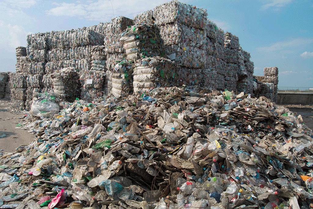
At six billion and climbing the human population is having a profound effect on our planet. We generate enormous quantities of materials and much of this ends up as waste. It is estimated that the average American creates over 1300 pounds (590 kg) of trash every year. What to do with this waste is an issue of public concern.
Plastics
Plastics make up some 9% by weight of the typical American’s trash. Most of this is in the form of used containers and packaging material. Historically this material has been used once and then sent to a landfill. Unfortunately, as the use of plastics for packaging has mushroomed, so has the demand for landfills. Recycling is now considered to be one of the best means to limit our need for new landfills.
But recycling poses a problem. Not all materials can be recycled in the same way. In prepping discarded plastics for reuse each distinct kind of plastic must be handled differently. Before plastics can be recycled they must first be separated into homogeneous piles. Such separations are a common problem in chemistry. The solution is to take advantage of the differences in properties of different materials to achieve a separation.
Measurement
Prior to the 17th century, chemical discoveries were based on observations of phenomena. Measurement was a crude and little used tool. By the early 1700s, though, careful measurement had become an accepted experimental tool and rather quickly led to the development of modern chemical theories. Today, precise measuring devices are an integral part of both research and applied science. The correct interpretation of experiments requires both precise measurements and an understanding of the error associated with those measurements.
There are a number of techniques you will need to use for this experiment. They are listed here. Details can be found from the techniques page.
- Measurement reliability
- Percent yield
- Graphing
- Mass measurement
- Linear measurement
- Volume measurement
Techniques
The following techniques will be required for this experiment. You will need to be familiar with them to successfully perform this experiment.
Mass Measurement—you will need to accurately mass the primary standard, KHP.
Linear Measurement—you will use a Vernier caliper.
Volume Measurement—pay particular attention to the use of the buret. You should practice using the stopcock with water before adding any reagent.
Data Manipulation—for this experiment the material on basic math, measurement reliability, percent yield and graphing are all pertinent.
Mass Measurement
In a chemistry lab, the mass of an object is determined by massing with a balance. If little or no accuracy is required, this is a rather trivial procedure. If a great deal of accuracy is required, it can be quite complicated.
Some issues to consider when trying to accurately mass an object.
- A wet object is heavier than a dry object. For example, a damp beaker can easily weigh 0.01 g more than a dry one. in addition, the weight of a damp object will change with time as the water evaporates. If you place an object on a balance and notice that the weight continually drops, there is a good chance the object is wet. This could limit the accuracy of the measurement to 0.01 g or less, depending on the amount of water present.
- A dirty object is heavier than a clean object. 0.001 g of dirt is not much dirt. For lab purposes, dirt is any unaccounted-for material such as dust, old labels, pieces of glass, grease, etc. Even visually small amounts of dirt can be a real problem if the object is weighed more than once. Dirt that comes off the object between weighings will adversely affect results.
- Fingerprints have weight. Fingerprints can weigh 0.001 g. Getting fingerprints on objects will invalidate the weighing at the 0.001 g level and must be avoided for accurate weighings.
- Hot items. Objects weigh less at higher temperatures. Even a moderately warm sample can weigh 0.001 g less than at room temperature. This is because the object heats the air above it, reducing the density of that air. The balance is zeroed against the room temperature air above the pan. The hot air weighs less and upsets this balance.
The balance itself must also be considered. The reliability of the balance will depend on its cleanliness. Dirt and chemicals that get inside will have unpredictable effects. Chemicals, in particular, can react with the balance, causing corrosion and reducing its life span. To ensure that our balances give you reliable masses and to preserve them for future students, the following rules govern the use of balances.
- Balances should not be moved. If you feel the urge to do so, consult a lab instructor. Every time a balance is moved it needs to be recalibrated.
- Nothing but glass or metal objects should ever be placed on the surface of a balance. Chemicals must never come in contact with the balance pan or any other part of the balance. For this reason, most of the weighing you do will be weighing by difference. In this technique, a container (beaker, weighing paper) is first weighed and then the material is added and the weight measured again. The weight of the material is the difference between the two weights.
- The balance should be cleaned after use. Chemical spills must be cleaned up immediately. If you suspect that chemicals got inside the balance, report it to an instructor so that the balance can be properly cleaned.
Weighing vs Massing
The terms “mass” and “weight” have different meanings, yet are often used interchangeably in a chemistry lab. Mass is a property of matter and is the term used to describe the amount of matter in an object. Weight is the force exerted by an object in a gravitational field. As long as the gravitational field is constant, mass and weight are directly proportional.
A balance is a device that compares the mass of an unknown object with the known mass of another object (or set of objects). Ironically, these known masses are referred to as “weights.” A scale is a device that measures the force exerted by an object due to gravity; in other words, its weight. Over time, the use of these terms has become very confused. It is common practice to say that “the weight of the beaker was determined to be 123.52 g.” Technically, if the measurement was made on a balance, it would be more correct to say “the mass of the beaker was determined to be 123.52 g.” Likewise, laboratory instructions often direct you to “weigh” objects. It would be more correct to direct you to “mass” the object.
All of this is admittedly very confusing. It is also not relevant to working in a chemistry lab. For the experiments you perform in this course, you can assume that the measured weights of samples are equivalent to their masses for evaluation purposes. When you are asked to “weigh” an object, you are to determine its mass using the available balance or scale.
Weighing a solid object that holds its shape (e.g., a beaker) is straightforward. The object is placed on the balance pan and the weight measured. Other situations may be more complicated. Here are some of the more common ones.
Weighing chemicals. Since chemicals must not be put directly on the balance pan, weighing by difference must be employed. Weighing paper is used to weigh chemicals that will be transferred to another container. This is a plastic-coated paper that chemicals will not adhere to. After weighing, the entire mass can be slid into a container. First the paper is weighed. Then the paper and chemical are weighed. The weight of the paper is subtracted to obtain the weight of the chemical. Some balances allow you to tare a container. To tare is to adjust the balance to read zero with the container on it. Electronic balances can be tared with the push of a button. Another suitable container is a beaker or flask. If the chemical is to be used in a beaker or flask, it is best to make the weighing directly in the container. First weigh the container, then add the chemical and weigh again. The weight of the container is subtracted to obtain the weight of the chemical. Again, it may be possible to tare the balance with the container on the pan.
Weighing liquids. The problem is similar to that of weighing a solid chemical. The solution is the same. Weigh an empty, dry container. Add the liquid and weigh again. Subtract the weight of the container to get the weight of the liquid.
Weighing by subtraction. Sometimes we’re not sure how much of a chemical we’ll be using, but we still want an exact weighing. Weighing by subtraction addresses this problem. The maximal amount of chemical is estimated. A container is prepared with this amount of chemical plus a little extra. The container and chemical are weighed. Chemical is removed and used as needed. When done, the beaker and left over chemical are weighed. The difference is the weight of chemical used.
Procedure for Weighing with an Electronic Analytical Balance
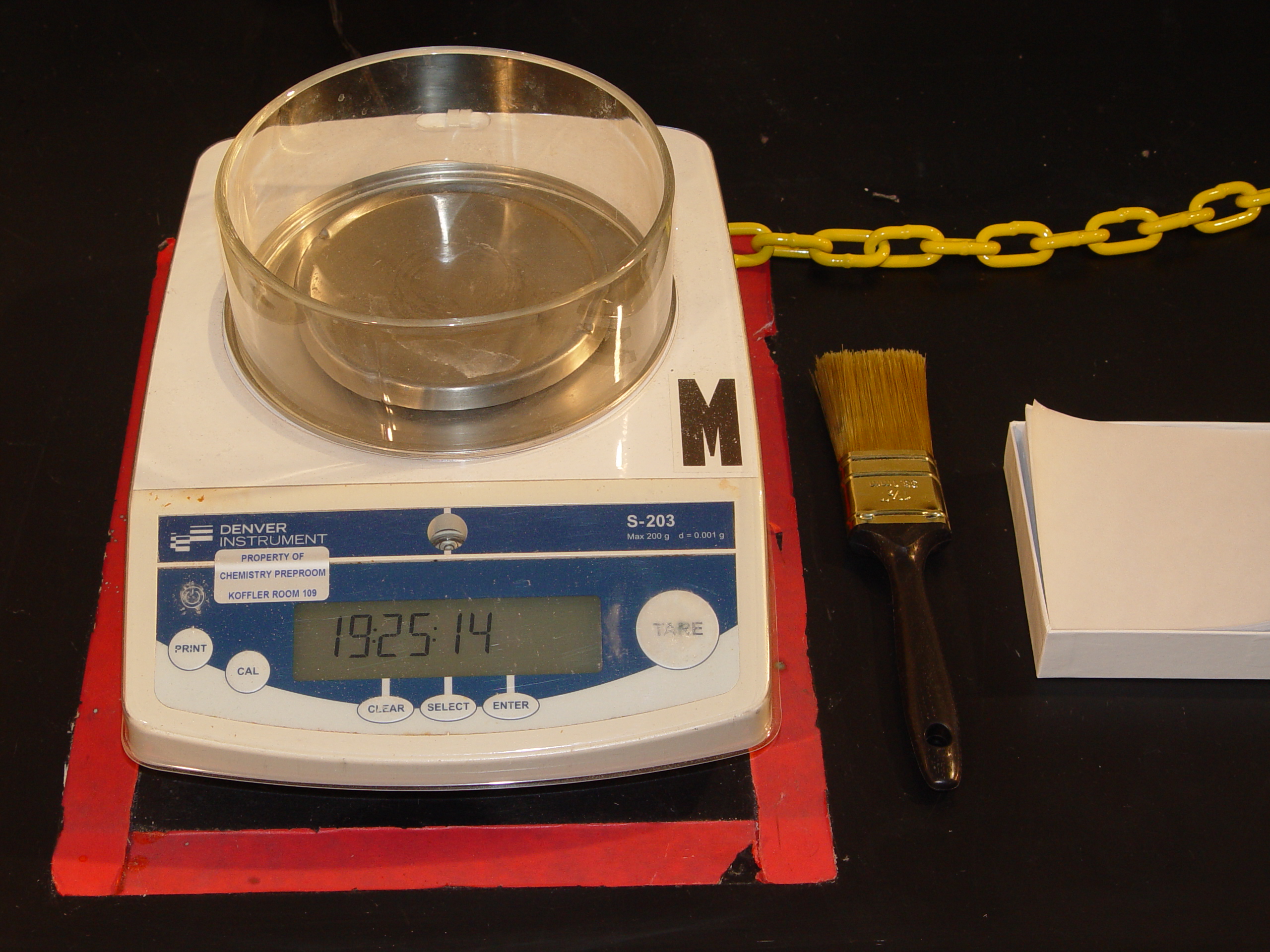
The electronic analytical balance is capable of measuring mass to the nearest milligram (.001 gram) or less. It is quick and reliable. It is also expensive and sensitive. It operates by measuring force. The pan is connected to a metal ribbon in such a way that a weight on the pan is mechanically translated into a torque on the ribbon. A stepping motor is also attached to the ribbon. The balance measures the voltage that must be applied to the motor to just balance the torque on the ribbon. This voltage is then electronically converted to a mass value that is displayed.
Because there are no moving parts, the balance is less sensitive to motion and shock than other balances. Because of the electronics, it is very sensitive to chemicals, particularly liquids and gases (fumes). Chemical spills can easily destroy one of these balances.
The balance is operated with control buttons. Different models have different arrangements. There are two controls you need to identify to use a balance. One is the ON-OFF button. The other is the zero control. This will usually be labeled as zero, re-zero, tare, or 0/T. Its function is to set the scale display to 0 g when there is nothing on it.
Using the Balance
- Check the pan to see if it is clean and dry. If not, clean it and dry it. If the balance has doors, close them.
- If the balance is off, press the on/off button. The balance will go through a self-calibration procedure that will last a minute or so. Wait for the display to fill with zeros.
- Press the tare button. Again, wait for the display to fill with zeros.
- Place the object to be weighed on the pan.
- Wait for the display to stop changing, then read and record the value.
- Remove the object. Clean the pan and surroundings. Leave the balance on unless instructed otherwise.
Please view the following "Using a balance" video clip.
Linear Measurement
The term “linear” refers to one dimension. A linear measurement is the measurement of the length of an object in one dimension. Linear measurements made in two dimensions allow for the determination of area and in three dimensions yield volume. The most common tool for measuring length is a ruler and you are probably quite familiar with its use. What you may not be familiar with is making and recording values that accurately reflect the accuracy of the measurement.
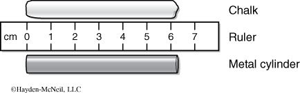
Consider the piece of chalk shown in Figure 1-1. Due to the irregular ends, the best reading is that the chalk is 6 cm long. Now consider the metal cylinder. It is more regular and we can more accurately read its length. In fact, we can estimate the distance between the marks on the ruler and come up with a more accurate reading. It is right and proper to read the length of the metal cylinder as 6.3 cm even though the ruler is marked only in centimeters. Such approximation is common in science and expected when using measuring devices. In this case, the edge of the cylinder is estimated to be 3/10 of the way between the 6 and 7 cm marks.
Vernier Caliper
A caliper is a device designed to accurately measure linear dimensions of irregular objects. It consists of two jaws fixed onto a ruler (see Figure 1-2). The jaws are brought together against the object to be measured. Most calipers have two sets of jaws—one for measuring outside diameters and one for measuring inside dimensions.
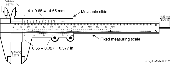
A Vernier caliper is a caliper with a Vernier scale attached. The Vernier scale provides a more accurate way to measure the distance between two closely spaced marks. The Vernier scale, located on the movable jaw, has marks that are 9/10 of the distance of the marks on the fixed scale. To read a Vernier caliper you align the jaws on the object to be measured and read the fixed scale at the 0 mark on the Vernier scale. If the 0 mark is not exactly over a mark on the fixed scale, you read the lower value off the fixed scale and then locate the mark on the Vernier scale that lines up with one of the marks on the fixed scale. This becomes the next value beyond the value read off the fixed scale. Consider the example illustrated in Figure 1-3. The reading is 160.4.
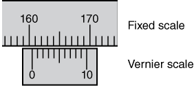
Please view the following video clip on “reading a vernier caliper”.
Volume Measurement
Volumetric measuring devices are very common in our world. Most kitchens have measuring cups and spoons. A volumetric measuring device is any container that will contain a known volume when filled to the mark. When making a volumetric measurement, there are two issues that determine how accurate the measurement will be. One is the accuracy with which the device was calibrated when it was made. Molded plastic and glass containers will only be as accurate as the machines that make them. The more accurate the device, the more expensive it will be. Common kinds of laboratory volumetric devices and their accuracies will be discussed below.
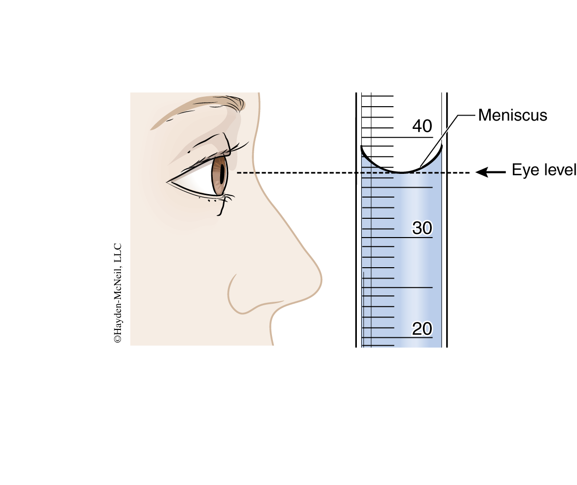
The other issue is determining when the surface of the liquid is at the mark. When a water solution is poured into a glass container, it “wets” the sides of the container. The resulting curved surface is known as a meniscus. All volumetric glassware is designed to be read at the bottom of the meniscus. When reading the meniscus make sure your eye is level with the meniscus.
When reading volumetric glassware, you should always estimate the value to one more significant figure than the smallest marks on the device. In the example pictured in Figure 1-4, the bottom of the meniscus falls between the marks for 36 mL and 37 mL. By visually proportioning the position of the meniscus between the two marks, the value of 36.5 mL is obtained.
When measuring a specific volume of solution, add solution to the container until the bottom of the meniscus just touches the appropriate mark. In this case the volume is read to one more significant figure than the mark. For example, if the bottom of the meniscus in Figure 1-4 had been just touching the 36 mL mark, the volume would be read as 36.0 mL.
Here are brief descriptions of the various devices commonly found in the lab.
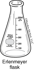
- Beakers and Erlenmeyer Flasks
These are designed to hold solutions and not for making measurements. The accuracy of the markings on a beaker is usually only ±10%. Beakers and flasks can be used for approximating volumes when accuracy is not required.
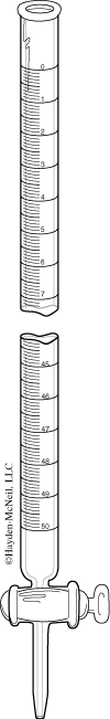
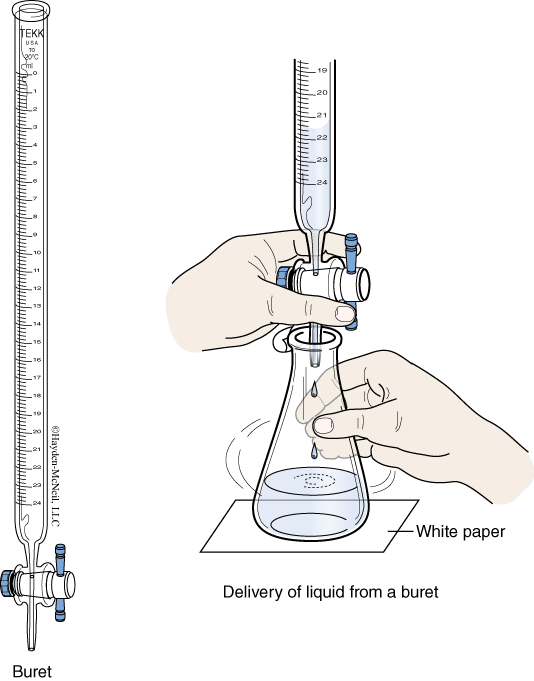
- Burets
A buret is a long, calibrated tube with a valve (called a “stopcock”) on the bottom. Burets are designed to deliver a variable amount of solution to the nearest 0.01 mL when used properly. Some things to consider when using a buret. - Operation of the stopcock can be tricky and requires practice to do quickly and reliably. For starters, the buret should be held upright with a clamp leaving both hands free to work the stopcock. Hold the body of the stopcock with one hand while turning the valve with the other. With practice, you should be able to deliver single drops with a buret.
- There is a dead volume at the bottom of most burets. If the liquid level falls below the last marking, an accurate reading will not be possible.
- Before use, a buret should be rinsed with some of the solution that will fill it. This is to prevent dilution errors that will occur if the inside of the buret is wet.
- All air must be removed from the buret. Any air present is volume that does not contain solution. This could very well lead to volume readings that are too large. There are two places where bubbles can be found. In the buret tube they tend to cling to the sides. Tapping the buret to dislodge them usually works. The other place is in the stopcock. After filling the buret, run solution through the stopcock until all air is removed.
- If a drop of solution remains on the tip of the buret, its volume will be measured but not delivered. There should be no drops of solution on the tip at the start or at the end of the measurement.
- It is considered bad form to try to fill a buret to a particular volume. The action of trying to exactly fill it could bias your results. Instead, you should fill the buret then read the volume.
- The position of the meniscus in a buret can sometimes be difficult to read. One thing that helps is to draw a straight, dark line on a white piece of paper (an index card is ideal). This is held behind the buret with the black line behind the meniscus. The white background and reference line should help you read the volume in the buret.
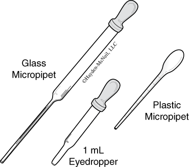
- Eyedroppers
These are small glass or plastic tubes designed to deliver very small volumes of solutions. They come with detachable rubber bulbs. Although they normally have no markings, they can be calibrated and used for volumetric measurements. To calibrate an eyedropper, count the number of drops required to add 1.00 mL of water to a small graduated cylinder. An eyedropper normally has a drop volume of about 0.050 mL. The rubber bulbs have a limited lifetime. As they age they get hard and brittle. Eventually they will need replacement. - Micropipets and Transfer Pipets
These can be either glass or plastic. The glass ones are like eyedroppers in that they have detachable rubber bulbs. A glass micropipet normally has a very long, thin snout (for getting into test tubes) and a drop volume of about 0.031 mL. The plastic ones are usually one molded piece of plastic. Sometimes they will have markings on the sides that allow for one significant figure measurements.
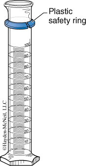
- Graduated Cylinders
A glass cylinder with calibrated volume markings on the side designed to measure the volume of liquid contained. The accuracy depends on its size. For small graduated cylinders it is usually 0.1 mL.
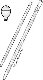
- Pipets
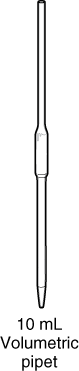
Volumetric Pipets
A glass or plastic tube used to accurately deliver specific volumes. A volumetric pipet has only one mark on it. When filled to this mark, the pipet will contain the indicated volume to the nearest 0.01 mL.
Graduated Pipets
A glass tube with a series of volume markings. Solution is drawn up into the pipet with a pipet bulb to a level above the desired mark. The bulb is removed and the end covered with a finger. The solution is allowed to drain away until the meniscus is at the correct mark. The pipet is now positioned over the receiving vessel and solution allowed to drain until the desired volume has been delivered. The markings on a graduated pipet usually don’t go all the way to the end. Thus, this kind of pipet will always have some solution remaining after use. Graduated pipets are designed to deliver solutions to the nearest 0.01 mL.
(Applies to both volumetric and graduated pipets.)
- Rinse the pipet with a small amount of the solution to be measured.
- Using a pipet bulb, draw solution up into the pipet to a level above the mark.
- Remove the bulb and cover the end of the pipet with a finger (it may help to wet the finger to make a good seal). Roll the finger, allowing solution to drain away until the meniscus is at the mark.
- Position the pipet over the receiving container and allow the contents to drain.
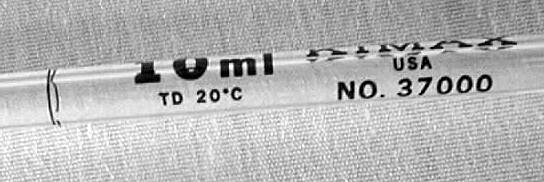
If the pipet has a small TC printed on it, it is designed “to contain” the specified volume. This means that the small amount of liquid remaining in the pipet is part of the measured volume. These are usually graduated pipets (see above) and require two readings (before and after). If the entire volume is to be used, all solution needs to be blown out of the pipet into the receiving vessel. Use the pipet bulb to do this.
If there is no marking on a pipet, you should assume it is designed to deliver.
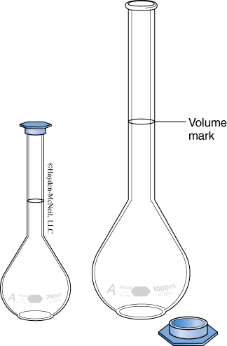
- Volumetric Flasks
This flask has one mark on its neck. When filled to the mark, the flask contains its design volume to the nearest 0.01 mL. Notice that this is a “to contain” and not a “to deliver” device. This is the most accurate volumetric measuring device presented here.
Laboratory Data Manipulation
Here you will find discussed a number of techniques for data collection and analysis that you will use frequently in this course. You may already be familiar with this material from previous courses. If so, then this chapter should provide a handy reference during your lab work. If this material is not familiar to you, then you will need to learn it before beginning lab work.
- Math assessment exercise
- Basic math
- Measurement reliability
- Percent yield
- Graphing
- Using Excel
Math Assessment Exercise
To be successful in a chemistry lab you will need to have certain math skills. This exercise is designed to help you determine if you have those skills. To perform the assessment, time how long it takes for you to answer the following questions. Then check your answers against those given at the end of the chapter.
- If you can answer all questions correctly in 30 minutes or less, your math skills are sharp and this chapter will be a review.
- If you struggle to answer some questions and it takes you longer than 30 minutes, you should expect to reference this chapter when writing reports.
- If you can not answer the questions, you should expect that you will require significant help with the reports and tests.
Question 1.1
jTDE6EJBU/QOyUZiP9jPYU16MN0kemIsKjD7oRTYWG1nSYz2kf3tNkPLEQPDuXMTQuestion 1.2
xwrYYCBS2WRUcohYhIo3/tUlobcQ4FxW8h2t7etCQVbBWuHQMG/zI/tZKUZ3/DYbSEDUiSR5MzJZS56VkyXdbkHPcLk=Question 1.3
rg73UYM1gSw/KUgt5NEJMDDkiNJMyoP9FboF0kiRg0Gc4k4JM7vd1IWxomav1z1+UjcE2w==Question 1.4
Ih279jak5bF+j78i8TOHj6uElZl9zGNGKCg7cilNLaip9RlhmzornaT/B1qQepw0EiwLUw==Question 1.5
zBeIz1uC1EQxSt0SVBMNFHBypFeKrXgL6LU66FvnCNvCQzfu0TichC9sgC8yHkK9of8cv8cXAVY=Question 1.6
f9y86TUiEYKtNep1hRbMXmDEcADHpMsSsz/fsXrI5Q7RamzO2EIO0q3t2B7VIp1Jwf4mJpSC6SAz+lye+6rBeJDL6o5+C1JvoIO8dYfWk9ulEB4maKtr+sLMqFWyqL6kQuestion 1.7
rJBqYyLUUEjN/IFRvWmRAf4yg+SY3CrxCDdf18ypAmZI4IQknjGgl1+NSSHAVILlc2j2Dg==Question 1.8
rk2r4J109SYtXmTYcQsdSaO/h3/1WJmUEEcfZCRSAPjqjWPyRj6P6dahrVfiPRwbsNVjt+A42JZM43c56oRnl2Vx//TQXIKQHoWFnZDs7fBnyJpfFQRgm9ZhXvcvrRB+xIqBQrAjRUw0Q0WB5Dpf/cyIiO7/M5KXhI5UvipOjfsN6gSHEAM9EuaNjaL7wYoWitufxFqRoDXR7Qx1n6bDnw==Question 1.9
wdmhNa4/TwJi0P+crceT43q6NiDZ58L33WVZBZP5XtvF8VV2eaJUM9OT8VXyuyz3hcFVKXTuE1JDrjlA+0WNFfbo/ve6mpD6jqT03IV+EKNfuHhjc2FAuURiMKRzgYD2tI/DrX+cLHaOV/WZZuvl//240Cjse3tMOzdE2SsimOw=Question 1.10
lgyCF9UhbR6DUzJaJRnW0Dxet46kFojfKAn9Pvp5FZnb5tNs1i8IQ8/yA8rhIseC8n6O3cmOLf5RjoWlp6ndSXhGT7crzWZLEzMNr3GBvQq9SC9BYX5XChPKTP0z9BpuLNwA2A==Question 1.11
5UwHtrypEOyGP67EM9Aa7oKCyuQiv2U8vJjz452zk1vC60xVHokt6DAZSVTZQ7K54bds5uSaPRJazL83M7mSt1A5/7g=Question 1.12
Question 1.13
HwE27fSIAxsEt0sr079mwqfMzeQbGWDav/+pkQIORW5xW0A1JeYEnTwPdkfzag+MwzAhcIOByPm/5Ic7xUUIlsaeBSknwvhP4S9ES0VrT7vFDpKRk3Ypx8c8W+NPmPAQVZkxsw==Question 1.14
/kLJDVYbcEMhVOmiMnAqhVEQ9v+z8OEsBIA5K5WfY4f6eV1s2Lm4zi2755xUS7EqKu0FujPfFLe+pYmMrWyyFLnfjVS9rKzrbkfdHdP7/PgPryJ2YoNo4jBdU9qsTsRNh4cvsLtXFZ4=Question 1.15
5tVSbpfzzhrhWXxjBeKVlOsQg7TFEnGAH0pZfNo/Z/P0A9nzB6CpPqakXiXJKS6RFabHzf4MJZXO8DoNx6izBGeG3y20cDuiADAZ/Hy460dkjtU3RJDxPhbLIcRw6fPmLWEJzg==Basic Math
Basic Math Operations
Interpreting the results of a chemical experiment frequently requires the use of mathematics. Sometimes this is as simple as dividing two numbers to determine a percent yield. On other occasions, rather complex analyses are required, as with the use of integration to interpret kinetic data. The following is a discussion of the mathematical skills you will need to successfully complete this course.
Making Conversions
Many laboratory problems require conversion of one unit to another: dollars to cents, liters to milliliters, grams to moles. The easy way to make simple conversions is to use a conversion factor, a ratio that connects the given unit to the desired unit. The values and units in this ratio are arranged so that, on multiplication, the given unit is eliminated and the desired unit remains.
Conversion factors are obtained from a simple equality. For example, consider the conversion of 20 miles into kilometers (km). We know (or can find in a table) that 1 mile = 1.61 km. This relationship produces two conversion factors.
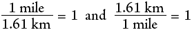
By multiplying the given unit, 20 miles, by the ratio, 1.61 km/1 mile, we get 32 km:
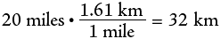
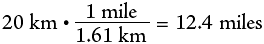
Note that 1.61 km is placed on top and 1 mile on the bottom so that the given unit, miles, can cancel, leaving the desired unit, km. If we want to convert 20 km to miles, we put 1 mile on top and 1.61 km on the bottom so that km would cancel, leaving miles:
More complex conversions will involve the use of multiple conversion factors. Any number of them can be strung together to obtain an answer with the desired units. This process is often referred to as “unit analysis” or “the factor-label method.”
As an example, consider how many dollar bills laid end to end would be required to circle the earth at the equator. First we need to know that the earth has a circumference at the equator of 24,000 miles and that a dollar bill is 15.5 cm long. The process will require converting miles to feet, feet to inches, inches to cm and finally cm to dollar bills. Here is how this is done.

Exponential Numbers and Scientific Notation
The last example demonstrates the problem of writing very large numbers. They take up lots of space and are hard to read. In chemistry we often deal with very large or very small numbers. For example, we say that 602300000000000000000000 atoms comprise a mole of atoms or that green light has a wavelength of .000054 cm. These numbers are rather inconvenient to use as written. To simplify calculations and reduce confusion, we use scientific notation. This is a shorthand notation that expresses all those place-holding zeroes as a superscript. The above numbers are written in scientific notation respectively as:

Algebraic Equations
An algebraic equation is a shorthand notation for expressing mathematical equality. For example, a researcher discovers that the mass of any piece of pure iron divided by its volume always gives the same answer, as long as all the pieces of iron are at the same temperature. Such a word description can be shortened to the following:

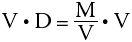
This expression can be simplified even further by use of symbols to give:

where M represents the mass of the iron, V represents its volume and D represents the constant number (known as the density). This is a simple algebraic equation. If any two of the above variables are known, the third can always be calculated.
You will use algebraic equations in this course to calculate unknown quantities. Occasionally you will need to rearrange an equation to use it. When attempting to determine the value of a particular symbol in an equation, it is necessary to isolate that symbol on one side of the equation (either side will do).
A general rule to remember is that you can perform a mathematical operation on one side of the equation (add, subtract, multiply, divide, square, etc.) as long as you perform exactly the same operation on the other side.
Example
Every substance has a constant value for density (D in the above equation) at a given temperature. Suppose we know the density of lead to be 11.3 g/mL. We wish to know the mass of a piece of lead but we can only measure its volume with the equipment at hand. Using the equation for density, we can calculate the mass in the following manner:

We wish to isolate the mass on one side of the equation. This can be done by multiplying both sides by the volume.
The mass equals the volume times the density. Therefore, multiplying the volume and the density gives the mass of the object.

Measurement Reliability
The Reliability of Measurements
Experimentation frequently involves making measurements of physical properties. Some measurements will be more reliable than others, but no measurement is absolutely correct. An understanding of the reliability of measurements made in the lab is crucial for the proper interpretation of the results of an experiment. This section will deal with a number of terms and concepts that you will need to understand to properly evaluate the measurements you make.
Experimental Error
In science, the term “error” has a different meaning than in general usage. To most people, an error is a mistake. Thus, “experimental error” is often interpreted as resulting from mistakes made by the experimenter. This is not always the case. The scientific definition of error refers to the uncertainty of results and not necessarily to the cause. Some sources of error are avoidable. Others are not. It is best to avoid thinking of error as “mistakes” but rather as uncertainty or deviations.
The Meaning of “Error”
A misconception regarding error is that it is bad. In fact, error is a property of all measurements. What is important is the magnitude of the error associated with a measurement. Whenever a measurement is made in the lab, the degree of error must be determined and then evaluated to see how it affects the interpretation of the results. For every experiment you perform, you must evaluate the errors associated with the measurements and discuss how they may limit the conclusions made.
Accuracy and Precision
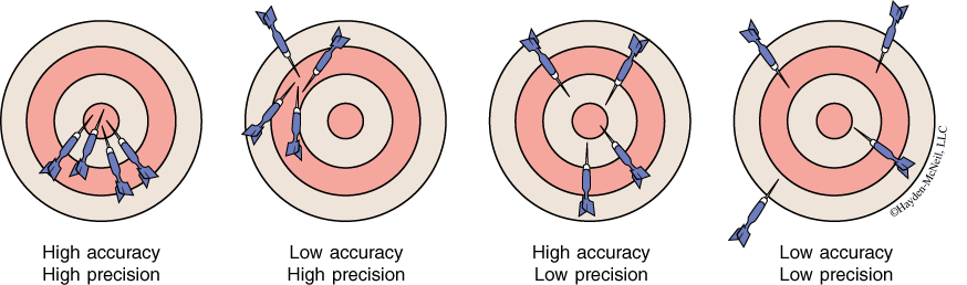
Accuracy and precision are two distinct ideas describing different aspects of a measurement’s reliability. Accuracy describes how close the measurement comes to the true value. Precision describes how close a series of measurements are to each other.
Accuracy and precision are relative terms. We normally talk of the degree of accuracy and the degree of precision. To say that a value is accurate implies a comparison to some standard. The standards are usually based on previous experience with the technique. Unless a verification experiment is being performed, the degree of accuracy of a measurement is determined by reference to the generally accepted accuracy of the technique and a subjective evaluation of the conditions of the measurement.
Since no measurement technique is perfect, repeated measurements of the same quantity usually show some scatter. The size of the scatter is a measure of the precision of the measurements (see Figure 1-5). In reporting the results of a set of measurements we should give the best value for the set. If all the measurements, are equally reliable, then the best value is the arithmetic mean, more commonly known as the average value. The average is the sum of all the values divided by the number of values. The mathematical expression for this operation is
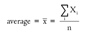
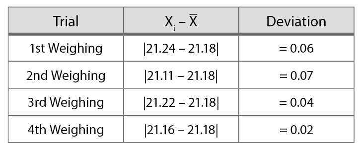
For example, suppose you weighed the same crucible four times and obtained the values presented in Table 1-1. The best value for the mass of the crucible is 21.18 g, the average of the four weighings.
Table 1-1. Crucible weighings.
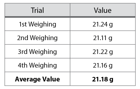
Clearly, this average value still has some uncertainty in it. After all, at no time was the mass of the crucible actually measured to be 21.18 g. Precision is a measure of the scatter in a set of data. The less the scatter, the more precise the data are.
Unlike accuracy, the precision of a data set can readily be measured. First, the deviation of each value from the average is determined.
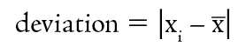
Note the absolute value bars. Deviations are always positive, regardless of the direction of the deviation. Table 1-2 shows the calculation of the deviations for the data in Table 1-1.
Table 1-2. Calculating deviations.
The deviations are inspected to determine if any of the measurements are questionable. A questionable measurement is one with a deviation significantly larger that the other deviations. Questionable measurements may need to be discarded. This would be determined by inspecting the lab notebook to see if any unusual events occurred that could explain the deviation.
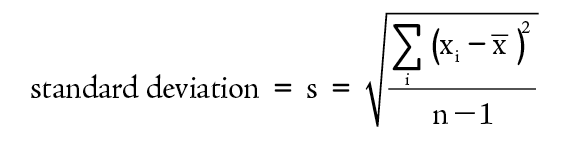
The deviations are then combined to produce a measure of the precision of the data set.
The most common method of expressing the precision of a series of repetitive measurements is the standard deviation. This operation produces a number that is a measure of how closely all values are clustered around the average value. In general, the standard deviation is a good predictor of the probable range of values that would be obtained from additional measurements.
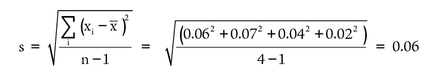
To see how the calculation of a standard deviation works, consider the data presented in Table 1-1. The deviations can be used as calculated in Table 1-2.
The precision of a quantity that was measured repetitively is usually expressed by presenting both the average value and the standard deviation. For our example, this would be reported as
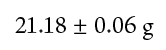
This representation gives us not only the best value for the measurements, but some indication of the uncertainty of the best value. In this case, the number 21.18 g for the mass of the crucible is uncertain to ± 0.06 g.
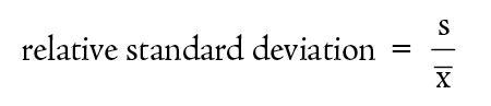
Another method of expressing the precision of measurements is the relative standard deviation. This is computed by comparing the standard deviation to the average value.
Relative standard deviation is most useful for comparing the precision of measured numbers that differ significantly in magnitude. For example, which set of measurements is more precise, a series of absorbencies that produces a value of 1.20 ± 0.09 or another set with a value of 0.341 ± 0.05? Is it the second set with the smaller standard deviation? Let’s look at the relative standard deviations.
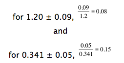
The first set of measurements is more precise.
Finally, relative standard deviations are sometimes presented as percent relative standard deviations. This is obtained by taking the relative standard deviation and multiplying by 100%. Thus, the above relative standard deviations become 8% and 15%, respectively.
Significant Figures
Anytime a measurement is made, there is a limit to the number of digits that can be read. This determines the number of significant figures for measurements made with that device. For example, a car odometer measures to the nearest 0.1 mile. With this device, a distance of 50 miles could be measured to three significant figures. When used properly, a 10 mL volumetric pipet measures ten-milliliter samples to exactly 10.00 mL, four significant figures.
The number of significant figures in a measurement will, in turn, limit the number of significant figures for any other numbers calculated using that number. As an example of significant figures, consider how reliably you can state your weight. If you say, “I weigh 160 lb.,” does this mean exactly 160 lb. or does it mean 160 ± 1–2 lb.? If you know your weight so reliably that you can say it is 160.000 lb., we say you know it to six significant figures. If you know your weight reliably enough to say you weigh 160 lb. ± a few ounces or so, we say you know it to three significant figures. In making calculations with measured quantities such as your weight, you cannot report your answer to more significant figures than is merited by the least reliable of the measured quantities used. For example, if you know your weight reliably to be 160 lb. and the volume of your body reliably to be 75 liters, you can calculate the density of your body by dividing your weight by your volume:
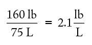
You cannot correctly report your density to more than two significant figures since the least reliable of the quantities involved in the calculation has only two significant figures. Thus you might correctly say that your density is 2.1 lb/L but you would be incorrect to say, on the basis of these numbers and calculations, that your density is 2.13 or 2.1333 lbs/L.
Percent Yield
In theory, all chemical reactions should give a 100% yield. In practice, this is not true. There are many reasons why the yield of a reaction will be different than 100%. The yield will be less than 100% if material is lost during the reaction or during the recovery process. It is also possible that the reaction itself did not go to completion. Yields that appear to be greater than 100% are also possible if the product is not pure.
In theory, a percent yield calculation is rather simple. You are comparing the amount of product obtained, the experimental yield, to the amount of product you predict you would obtain if the reaction were 100% complete and there were no losses.
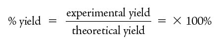
In practice, there are tricks to determining a percent yield. First, a percent yield is a ratio and can not have units. This means that the experimental yield and theoretical yield values must use the same units. Most commonly moles are used, but the calculation also works with grams.
To determine the experimental yield, the mass of product is determined. If the molecular weight is known, then this mass is converted into moles.

The theoretical yield is determined from the moles of product predicted based on the chemical equation. For this determination one must use the coefficients in the chemical reaction.


Graphing
The relationship between various experimental parameters is often best understood by graphing the data obtained. Sometimes a graph is needed to obtain the desired experimental result. The value of graphical analysis is strongly dependent on the quality of data used and the degree of care employed in constructing the graph. Graphs should be constructed in such a manner that they do not reduce the accuracy and precision of the data presented. The following graphing pointers are presented with this goal in mind.
1. Select Your Platform
Graphs can be made either by hand or using computer programs. Graphs constructed in lab will often be made by hand. It’s always a good idea to graph data as you go. This allows for the identification of problems as they occur. It is also sometimes necessary to graph data to determine what to do next. Final graphs intended for inclusion in reports or posters can be made by hand, but are usually better if generated using a computer.
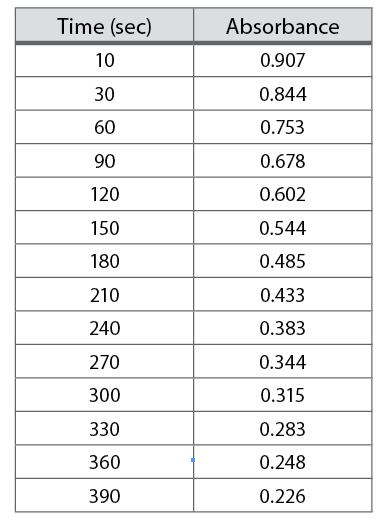
Table 1-3. Dye bleaching data.
Using a computer will void the need to use graph paper, but may generate other problems. If you are unfamiliar with the operation of the program you could end up generating an inaccurate or misleading graph. Conversely, computer generated graphs allow for more complex manipulation of data. Graphical presentations can be further analyzed to produce more convincing arguments. The choice of hand-drawn or computer-generated graphs will depend on the requirements of the particular experiment and the course.
2. Handmade Graphs
If you construct your graph by hand, you will need graph paper to ensure that your data points are as accurately placed as possible. The following discusses how to construct a suitable graph.
Select the axes. A two-dimensional graph will have two scales. The x-axis, or abscissa, runs left to right across the graph. The y-axis, or ordinate, runs up and down. Normally, the independent variable is plotted along the x-axis and the dependent variable on the y-axis. The independent variable is the one for which you set the value when you perform the experiment. The dependent variable is the data obtained as a result of your selection of the independent variable. Consider the data presented in Table 1-3. This data was collected by placing the sample in a spectrophotometer and then reading the absorbance at specific times. The time is the independent variable. The values were selected by the experimenter and will be placed along the bottom of the graph. The absorbance is the dependent variable. It was read from the machine at the chosen times. The absorbance will be plotted up and down.
Determine scale ranges.To ensure maximum usefulness of your graph, you need to select scales that will allow your graph to be as big as possible. Begin by identifying, for each range, the largest and smallest values in the data set. In Table 1-3, these are 10 and 390 for the times and 0.907 and 0.226 for the absorbance. Next, identify how many small divisions are available for each axis on the graph paper available to you. Finally, determine the nearest integral number of units per graph division. Once the values for each division have been determined, draw the axes on the graph and label some major lines with their values. See Figure 1-6 for an example.
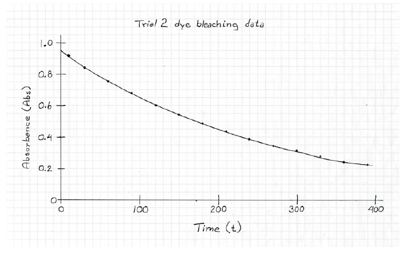
Plot the data. Place a small dot, or x, at the location of each of the data points. After all the data have been plotted, draw the smoothest curve possible through all your points. Do not simply connect the points.
Label the graph. The graph will not be complete until you have titled it and labeled each of the axes. Don’t forget to include the units. Again, see Figure 1-6 for an example.
3. Computer Made Graphs
These are ideal for the formal presentation of data if they present the data in the proper context and with sufficient detail. The first consideration is the suitability of the software. There are many graphing programs available with many different capabilities. A suitable program will allow the user to perform the same manipulations described for hand graphing. It will also allow for the interpolation of values, if required, with the same accuracy as the data used. The most common spreadsheet program is Microsoft’s Excel, which is discussed in the next section.
Using Excel
Excel is the spreadsheet component of Microsoft Office and is quite common. It is designed primarily for use with financial data but can be made to work for scientific applications. It is most useful for performing repetitive calculations on large data sets, for graphing experimental data and for generating professional looking results tables. The following is a brief and rather cursory introduction to some of the more useful features of Excel.
1. Basic Data Entry
The spreadsheet consists of data cells arranged in columns and rows. Columns are identified by letters and rows by numbers. Thus, the first cell in the upper left hand corner is cell A1. There are two ways to enter data into a cell. Select the cell then double click on it to get a cursor in the cell. Alternately, select the cell and type in the edit bar at the top of the spreadsheet.
If you enter a number Excel will treat it as a number. If you enter any character other than a number Excel will treat it as a label. Mixed numbers and letters are labels. If you wish to enter a number but have it treated as a label, start the entry with an apostrophe.
2. Basic Data Manipulation
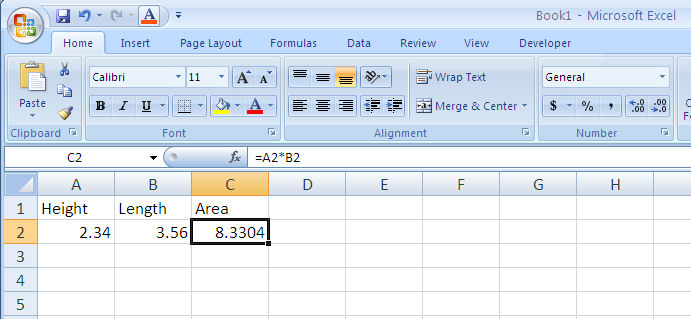
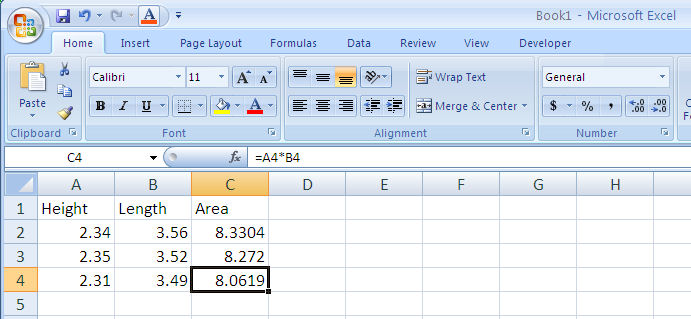
You can have Excel perform mathematical operations by using equations. To create an equation, start with an equal sign (see Figure 1-8). Excel recognizes standard operators: addition (+), subtraction (-), multiplication (*), division (/) and power (^). You can also nest calculations using parentheses. Notice that the equation appears in the edit bar.
3. Copying Formulas
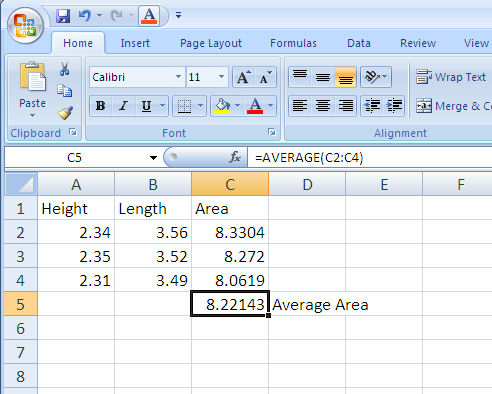
When you copy a cell containing an equation you will copy the equation. Excel will automatically change the cell references to correspond to the new cell you’re copying into (Figure 1-9).
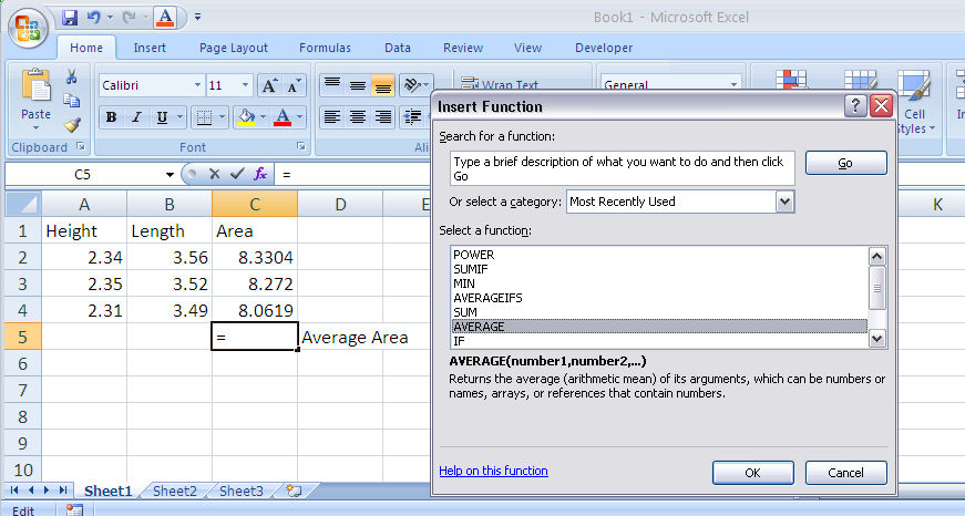
4. Using Functions
Excel contains many functions stored for your use in equations. To access the function menu double click on the fx symbol on the edit bar. A function consists of a function name followed by parameters in parentheses. The parameters are usually the cells to be included in the function calculation. For example, the equation for calculating the average area as shown in Figure 1-9 will be =AVERAGE(C2:C4). Note that the colon indicates an inclusive range of cells (C2 through C4).
5. Toolbars
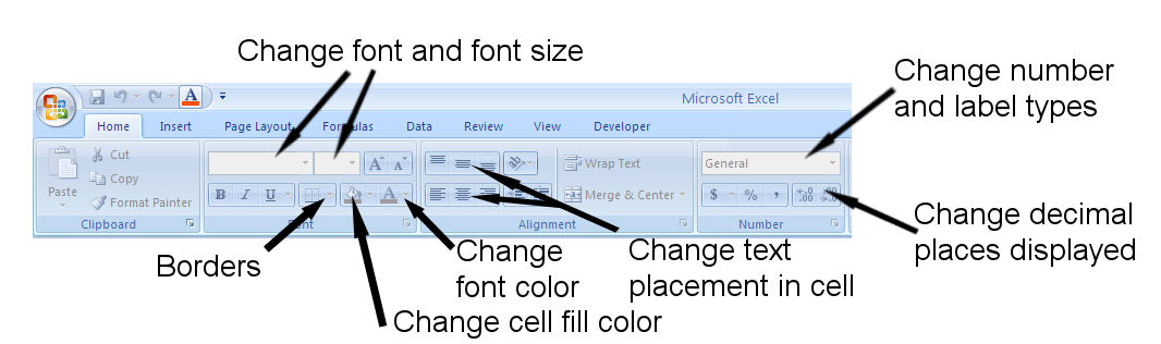
Figure 1-11 highlights some of the more useful features of the two most useful Excel toolbars. The rest of the buttons on the formatting toolbar can be used to format the contents of cells. Highlight the cells you want to format and then select the desired formatting function.
Chart Wizard—for making graphs and charts. This tool is discussed in the next section.
Change decimal places—for setting the number of decimal places displayed in a cell.
Create borders—for drawing lines around sets of data. Borders can also be created by selecting Format > Cells > Borders. In both cases borders will be drawn around the collection of highlighted cells.
One commonly used effect is to put labels in cells that have white text on a black background. You can do this by setting the fill color to black and the text color to white.
6. Graphing Data
Excel can graph columns of data. It will graph one column against one or more other columns. The organization of the data is critical to the appearance of the graph you produce. The following is a description of how to generate a non-linear graph using the Office 2000 version of Excel.
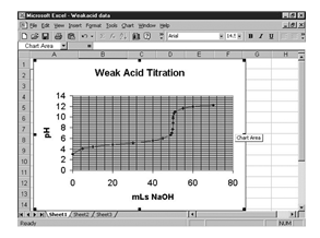
Consider the titration of a weak acid with a strong base. Small amounts of NaOH are added to a solution of the weak acid and a pH measurement is made after each addition. A tabular presentation of the data is recorded in the lab notebook (Table 1-4).
Table 1-4. Spreadsheet data.
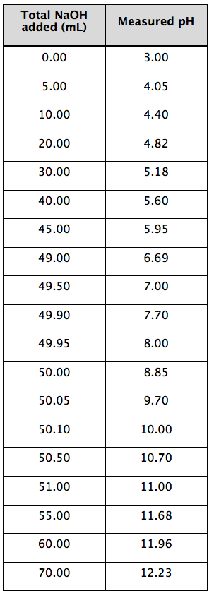
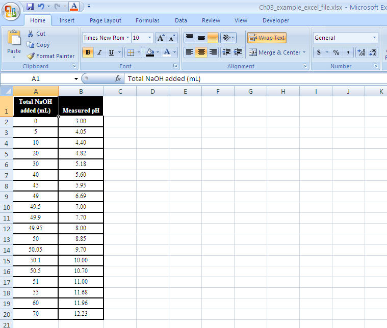
Enter data into spreadsheet. Copy the data into columns A and B of a blank spreadsheet. The independent variable (vol NaOH) goes into column A. It’s always a good idea to label the columns. Figure 1-12 is an example for the data in Table 1-4.
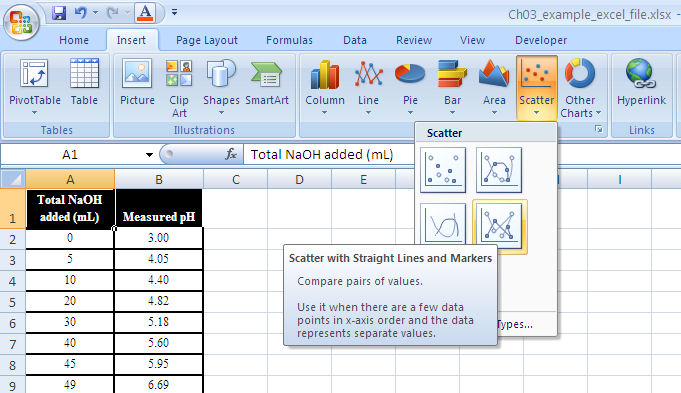
Setting up the graph. From the menu bar select “insert” and then “chart.” This should load up the Excel Chart Wizard which will guide you through the rest of the process. Alternately, you can choose the “chart wizard” icon from the toolbar.
Next, select the type of graph. For most applications the “XY (scatter)” and “scatter with data points connected by smoothed lines” are the most appropriate. (See Figure 1-13.)
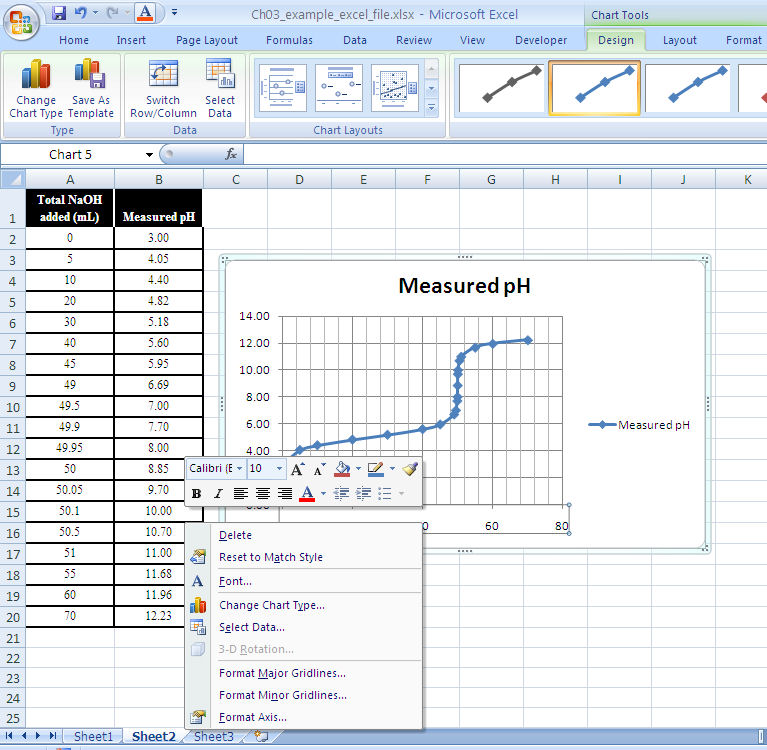
The Chart Wizard will show your data graphed. If the program did not select the data range, or if it is wrong, highlight the range you want graphed and enter it. (See Figure 1-14.)
The Chart Wizard will now ask you about gridlines. The number of gridlines will depend on what you need to do with the graph. If values are to be read, both major and minor gridlines for both the x- and y-axes are appropriate.
Finally, the Chart Wizard will ask you where to put the chart. Once placed, you can adjust the size and shape by stretching the eight “chart area” buttons. You can edit other graph parameters by right-clicking on the graph and selecting “chart options” from the menu. A screen will pop up allowing you to modify the titles, gridlines, legend, and data labels.
Procedure
This experiment requires you to work with a group. You are not expected to personally make every measurement described here. Rather, you and your group members are expected to collect a complete set of data. In addition you are to learn how to properly make mass and volume measurements. It is important that you personally make enough measurements to ensure this happens.
Density of a Known Plastic
Your group is to determine the density of a piece of plastic to the best of your ability. The tools available to you in the lab are: a milligram balance, a ruler and a caliper. The piece of plastic will be provided by your instructor.
Identify a balance to use. Examine the front panel and familiarize yourself with the controls.
Determine the mass of the plastic. Determine its volume via displacement. Also determine the volume by performing the required linear measurements and calculating the volume.
Calculate the density. Compare your results to those working with the same plastic.
Identifying Plastics using Mass and Volume Measurements
Your instructor will provide you with an unknown piece of plastic. Using mass and volume measurements, determine its identity.