Chapter 12. LAB 12 Models in Biology III: Population Growth
Learning Goals:
- Know the factors that affect populations and their growth or decline, and understand how we acquire information about these factors
- Understand the effects of environmental factors on bacterial populations, as well as compare in vivo bacterial growth with models
- Understand why models are important tools in population ecology, the different types of population models used by scientists and the benefits and disadvantages to using each type
Lab Outline
Activity 1: Measuring Population Growth in Escherichia coli
Activity 2: RAMAS EcoLab
2A: Exponential Growth in Bacteria
2B: Growth of Human Populations
Scientific Inquiry

Three thousand years ago there were approximately 50,000 people on earth. Three hundred years ago there were approximately 700,000. Today, the world population is estimated at 7 billion (US Census Bureau 2012). Why did the population increase by two orders of magnitude in the first time period and four orders of magnitude in the second? What determines how quickly a population grows, and whether it continues to grow indefinitely? Will it ever reach a plateau? Four factors determine whether a population grows or shrinks: births, deaths, and movement into or out of a population (immigration and emigration, respectively). These factors are influenced by both biotic factors such as competition, predation, and disease and abiotic factors, such as temperature and humidity.
All of the organisms of a single species living in one area constitute a population. An understanding of populations is an important one in our study of living systems. We can speak, for example, about the spotted owl population in the Pacific Northwest or of the bacterial population in your mouth right now. Populations, like organisms, may grow or diminish in size, move over a geographic range, consume resources, and interact with other populations. Just as an entire organism is made of individual cells and has properties that the cells do not, a population has unique characteristics and functions different from the individuals within the population. Similarly, populations are able to evolve (through natural selection and other processes), while organisms cannot. Since there is a distinction between a population and the organisms that make up the population, it is important for us to gain an understanding of how populations, not just organisms, behave.
What makes research into population growth important?
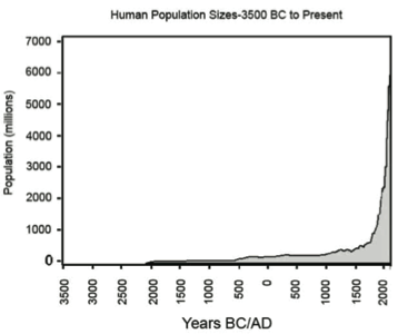
Consider human populations—Figure 1 shows how the human population has grown. In 2008, there were approximately 6.6 billion people living on earth and eighty-two percent of us are living on only 10% of the land’s surface. For most of our history, our population grew slowly. But in the past three centuries that stability has been interrupted by a series of growth surges. Several factors have been cited to account for a rapid increase in population growth. One factor is the improvement in food production both in quantity and quality. Other people cite as a an important factor the vast improvements in health and medical practices due to the discovery of bacteria as an agent of disease, which caused the death rate in the human population to fall drastically. This, along with other improvements in quality of life during the Industrial Revolution (mid-to-late 1800’s) led to a spike in the human growth rate. It is estimated that there will be more than 9 billion people living on earth by the year 2050, consuming even more resources on an already stressed planet (US Census Bureau 2012, United Nations 1999).
Background
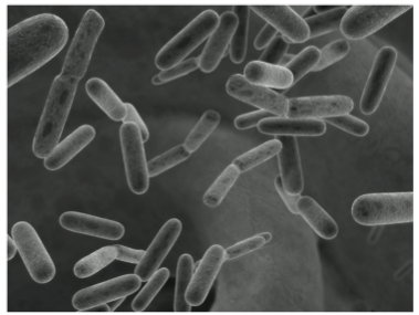
There are two major approaches to studies of population growth—one approach uses data collected from living populations, the other approach uses computers to track hypothetical population sizes according to a prescribed mathematical model, which may or may not be based on population data. We will use both of these approaches in lab. Small samples of live bacteria will be cultured in lab using different bacterial growth media—we will monitor their population sizes during lab. Under optimal conditions, the E. coli bacteria (Figure 2) used in these experiments are known to divide by mitosis once every 20 minutes—one cell divides to form two cells, twenty minutes later two cells become 4 cells, etc. Think of the implications —a single bacterium dividing every 20 minutes will give rise to over a thousand bacteria in a mere ten cell division cycles—do the math. Thus, within a single laboratory period we should be able to track changes in bacterial population sizes over multiple generations.
Since we know the doubling time for E. coli under optimal conditions we can make a simple mathematical model of bacterial population growth over multiple generations. We could do these calculations on our own but instead we will use a population modeling software called RAMAS which will save us time by allowing us to simply input the doubling time of an E. coli population and a given starting number of individuals—RAMAS will calculate and graph changes in population sizes over time for us using a mathematical equation that describes logarithmic growth. Although RAMAS can track populations that just double in size over time using simple mathematical models, it can also input complex algorithms or mathematical equations to track populations whose growth rates are complicated by changes in birth and death rates, and by immigration and emigration. In today’s lab, data from our living bacterial population growth will be compared and contrasted with RAMAS computer simulation graphs.
Microbiology Refresher
E. coli bacteria are commonly used in DNA technology labs for transformation, cloning, and plasmid purification. In today’s lab, these bacteria will serve as the experimental organism in population growth experiments using different growth media as experimental variables.
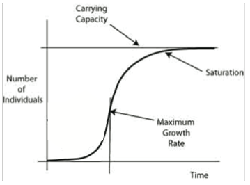
You will start with a culture of E. coli cells grown overnight to saturation (Figure 3), that is, the population has reached its stationary phase at a high population density. Because the culture at saturation is very dense and the carbon source almost depleted, we must dilute them into fresh media to insure that they are able to grow at maximal rates in our population experiment.
The graph in Figure 3 shows the changes in growth of a population over the time it takes for a population to reach carrying capacity. During the exponential phase, at the ascending linear portion of the curve, growth rate is maximal. The initial flattened portion of the curve is called the lag phase and is not linear. During the lag phase the bacteria are synthesizing materials, like RNA and enzymes, to allow for maximal growth during the rising exponential growth phase. The cells reach stationary phase when nutrients are limited and death rate usually equals birth rate. The death phase follows this, when all nutrients are depleted and the waste products are high. The curve begins to slope downward for the death phase. The stationary phase can last a very long time. Most cells used in molecular biology are grown to saturation (i.e. stationary phase) and are then diluted for further use.
High densities of bacteria make their culture media cloudy. We can use cloudiness, also known as turbidity, as an estimate of bacterial population sizes by measuring the amount of light blocked by the bacteria—as the bacteria divide and grow their increasing density results in increasing turbidity. Spectrophotometers are made to measure the amount of light that passes through a cloudy solution providing information about the cell density of our bacterial population—the greater the absorbance reading in the spectrophotometer, the larger the bacterial population. Absorbance is known conventionally as optical density (OD) when the length of the path of light through the sample is 1 cm. A value of OD = 1 at 600 nm for a culture of E. coli approximately corresponds to a concentration of 1.0 × 10⁹ cells/ml (Bionumbers 2010). Although this estimate varies depending on the particular strain of bacteria, you will use this conversion to monitor the changing population sizes of your E. coli.
An Introduction to Modeling
The ability to model a life process using mathematical equations or conceptual frameworks is a valuable skill in biology. Models allow researchers to forecast and predict empirical data (climate change, for example). By paring a system down to its essential parts, models can give researchers a pattern to look for where none was visible before by pointing out key components of the system. A model may serve as a starting point or simplified hypothesis. However, this simplification can lead to problems. One of the biggest problems with models is that they often do not contain enough reality. Biological systems are complex. In order to weed out “noise” in the data that is irrelevant to the experiment, a model may leave out details that may be important to understanding the system in its natural context.
Models are an example of scientific reductionism where a relatively large life unit is studied as a series of smaller parts. For example, the human body is a life unit composed of numerous organ systems, cardiovascular, digestive, muscular, nervous etc. When doctors specialize in different organs or systems—they reduce the human body to separate systems that contribute to the overall functioning of the whole body. By knowing details about heart function, a cardiologist provides insight into the health of a patient’s heart. However, restrictive models can be used to clarify and simplify a complex system or be misused by omitting or ignoring important aspects of the larger whole. When we only use information from one part of a larger system we potentially omit critical information from other essential systems—this may lead to faulty conclusions since a heart patient may be treated for cardiac problems but may have unrecognized illnesses due to dysfunction of different organs systems, such as the excretory or nervous system.
Will we be able to model our findings from the bacteria growth experiment in this lab? Although in theory it is possible, we should note several limitations of this experiment before we start. First, the bacterial culture in Activity 1 does not start with a single individual—there will be many millions of cells per milliliter in our starting cultures. We do expect to see a similar pattern of population growth but not similar numbers of bacteria in our model vs. actual data. Our model will assume that the rate of growth of bacteria is constant over time, although it is not. Our model will also assume unlimited food—is this an accurate assumption in our Activity 1 culture? The most important difference between Activity 1 and the model we will create is that our model will be deterministic; there is no environmental variability assumed in the model whereas our cultures contain both planned and potentially incidental environmental variability.
In Activity 2A, you will consider a hypothetical bacterial population whose model is based on specific input data—the initial population is a single bacterial cell and its generation time is 20 minutes. This means the individual undergoes asexual reproduction and produces two organisms in 20 minutes. These two individuals can, after an additional 20 minutes, each reproduce again resulting in a total of 4 bacteria. This process continues so that after each reproduction there are not just two more individuals, but double the number that were alive in the preceding time step. This is called exponential growth and displays graphically as a J-curve (Figure 1). Exponential growth may start slowly but growth accelerates astonishingly quickly under this model.
Do humans grow like bacteria? Can we model human population growth?
In Activity 2B, you will model human population growth using RAMAS EcoLab software and examine how different factors may influence human demography.
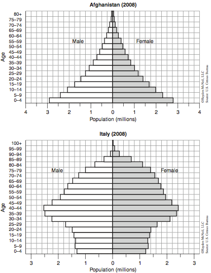
The population of the United States of America increases by about 1 percent each year. In 1993, there were approximately 265 million people living in this country. We can therefore expect that over two and a half million more individuals (equal to the number of people currently inhabiting the entire state of Kansas) were added to the population by 1994. It is interesting to note, however, that our country is not growing nearly as quickly as some others are. In fact, Afghanistan is growing 2.5 times as fast as the United States. On the other hand, Italy is only growing at one-tenth the rate of the United States (see Figure 4).
Age-structured models and the Leslie matrix
Compared to Activity 1, we will use a relatively sophisticated “age-structured model” in Activity 2B. In age-structured models, key concepts of survival rate (also called survivorship) and fecundity (the number of offspring produced in a given period of time) are presented as they change with age. For example, the fecundity of people between the ages of 20 and 29 is certainly higher than the fecundity of people between 0 and 9 years old. Likewise, the survival rate of humans changes with age, generally decreasing as we grow older. This is in contrast to the bacterial growth model in the last activity, where all individuals were assumed to have the same probabilities of survival and reproduction, regardless of age.
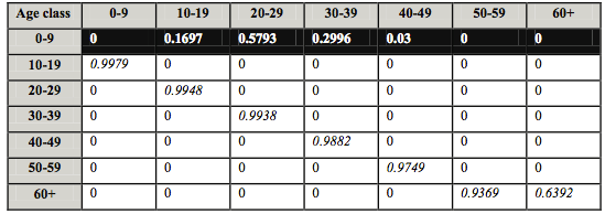
This age-structured model makes use of a Leslie matrix, which is basically a table of numbers; the fecundities are shown in the upper (black) row of the matrix and survivorship of each age class is represented on a diagonal across the table. In the following activities, the human population is broken down into the following seven age classes: 0-9, 10-19, 20-29, 30-39, 40-49, 50-59, and 60+. Here “60+” includes all people who are 60 years old and older. The Leslie matrix for this model is shown in Figure 5.
In general, an age-structured model may have any number of age classes. In this matrix, the white numbers in the top black row represent fecundities; the fecundity for age class 10-19 is 0.1697. This means that on average, each female in that age class has 0.1697 babies in a ten year time interval (notice that the time interval is the same as the length of each age class). Of course, no woman can have 0.1697 of a baby, so this really means that most women in that age class have no children, but the average is about 0.1697, or nearly 17% of 10-19 year old females have children.
The remaining non-zero numbers (italicized) represent survival rates to the next age class. The youngest age class (0-9 years) has the highest survival rate, 0.9979. This means that 99.79% of all children between the ages of 0 and 9 years survive into the next age class, which is 10-19. Similarly, 99.48% of children between ages 10 and 19 survive into the next age class (see that the survival rate is 0.9948). As you can see, survivorship declines as we get older. Although the Leslie matrix will be smaller or larger depending on the number of age classes, the general idea is the same; the fecundities run along the top row, and the survival rates run along the diagonal.
Note the value entered in the lower-right corner cell of the table. You might expect this value to be zero, since no one should survive past the last age class; there is no older age class. The value entered at the bottom right corner of the Leslie Matrix here is 0.6392 instead of zero since we are merging age groups 60 and above— this value is necessary for the RAMAS software to run since there must be a survivorship value in the last column but final age group in which there were no survivors.
Resources
Allan D. 2006. Population Growth over human history (lecture notes). http://www.globalchange.umich. edu/globalchange2/current/lectures/human_pop/human_pop.html Accessed 2013 July 1.
Applied Biomathematics. 2007. RAMAS. http://www.ramas.com/software.htm Accessed 2012 June 8. The RAMAS EcoLab portion of this laboratory was adopted with permission of Lev R. Ginzburg, Ph.D.
Milo R, Jorgensen P, Moran U, Weber G, and Springer M. 2010. BioNumbers—the database of key numbers in molecular and cell biology. Nucl. Acids Res. 38(suppl 1): D750-D753. http://bionumbers.hms.harvard.edu/ Accessed 2013 June 22.
United Nations. 1999. The World at Six Billion. http://www.un.org/esa/population/publications/sixbillion/sixbilpart1.pdf Accessed 2013 July 1.
US Census Bureau. 2012. US Census Bureau International Data Base. http://www.census.gov/population/international/data/idb/informationGateway.php Accessed 2013 July 1.
Lab Preparation

Complete the BioPortal Quiz, which is designed to gauge your understanding of the prerequisites for this course, as well as your knowledge of the required content. It is your responsibility to review this material, if necessary, then watch the vodcast and read this lab. Place all notes in your lab notebook, which can be used during the Pre-Lab Quiz.
Activity 1: Measuring Population Growth of Bacteria
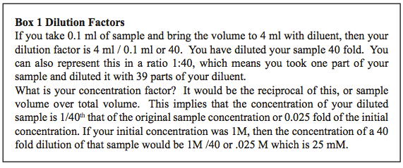
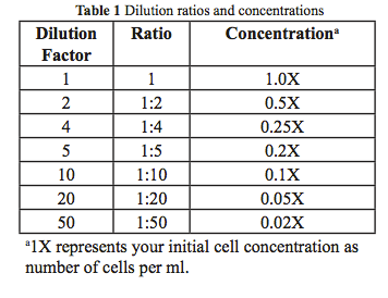
In this lab, bacteria will be used as the experimental organism in population growth experiments using different bacterial growth media as the experimental variables. You will dilute the stock culture so that the starting population density for your experiment is initially low and readable in the spectrophotometer. The dilutions will be made in small sterile flasks. Samples will be removed into 13 mm disposable test tubes for reading the absorbance of the cultures in the spectrophotometer over time. Recall that dilution factors are the final volume over the amount of the sample to be diluted. These simple relationships are explained in Box 1 and Table 1.
Make Predictions: What effects do you think the different media will have on E. coli? Write your predictions in your lab notebook. How do you expect absorbance or transmittance to change over time? If you see no change in absorbance, what factors could be responsible?
Learning Objectives
After successful completion of this activity, you should be able to:
- Use the Spec20, micropipettor, pH meter, and incubator
- Make and dilute solutions
- Dilute bacterial cultures
- Use aseptic technique
- Monitor organism growth and cell density using the Spectrophotometer
Materials
pH meters and thermometers
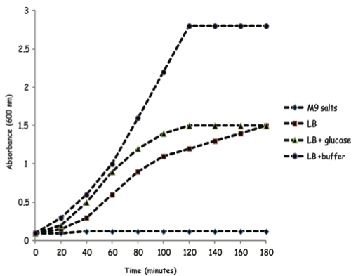
Growth media and reagents: M9, LB, glucose or other sugar, LB + phosphate buffer
Air shaker at 37°C and 200 RPM
E. coli culture grown to saturation in LB: strain ____________________
Culture tubes (13 × 100 mm)
Flasks
P1000 and P100 micropipettors and tips
Kimwipes
Solid and Liquid Biohazard Waste Containers
Waste beaker (for Kimwipes and tips)
Test tube rack
Parafilm, aluminum foil, marker, timer, and tape
Spectrophotometer
Vortexer
Turn on the Spec20 at the start of lab; let it warm up for at least 10 minutes before use.
Procedure
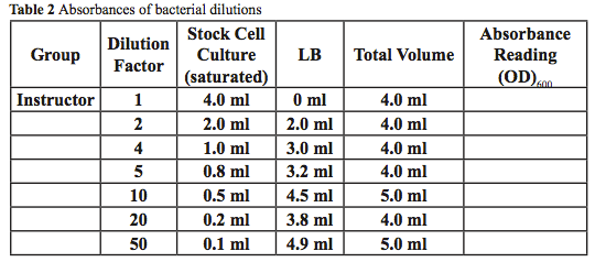
- Dilute your saturated cell stock according to the dilution assigned by your instructor. Each group will make one of the dilutions from Table 2 using the stock cells and LB media as the diluents. Note: You need to determine the dilution factor at which to dilute your cells before you can begin your experiment.
Does the absorbance increase or decrease the greater the dilution factor? Explain.
- Vortex the cells gently to mix the dilution.
- Blank the spectrophotometer and measure the absorbance of your group’s sample. Record your value in the class data table. Your instructor will read and record the absorbance of the saturated culture which should be >1.0.
- As a class, plot the dilution vs. the absorbance in Excel. At what dilution(s) does the absorbance fall between 0.1 and 0.3? ______________. Select the dilution the class will use for the experiments.
- Prepare a blank(s) appropriate for each flask in your experiment.
- Retrieve two sterile flasks and label them using tape. Based on the appropriate dilution, prepare your two flasks using a total volume of 20 ml according to the experiment (a, b, or c) assigned to your group. Your instructor will prepare cells grown in M9 salts and LB broth as controls and two groups will collect data on those cells. What type of controls are these?
- E. coli in LB + glucose
- E. coli in LB + buffer
- E. coli in LB + buffer + glucose
- Prepare four labeled glass tubes, two per flask. You will use two of these tubes to withdraw samples from your cultures in order to read their absorbance. Once you have prepared your cell dilutions, remove 2 ml of each culture into the properly labeled glass tubes. Set these tubes aside in the rack on your bench.
- Remove 4 ml of each culture into the remaining two glass tubes. Record their absorbance at zero time using the appropriate blank.
- Pour the 4 ml sample back into the correctly labeled flasks and recap the flasks with the double layer of foil.
- Place your flasks in the incubator set at 37°C and 200 rpm. Note the clock time.
- While your flasks are shaking read the starting pH and temperature of the two tubes you set to the side. The probe of the pH meter should fit inside the glass tubes.
- After use, rinse the thermometer and pH meter probe with the water squirt bottle over the biohazard waste beaker. Gently swirl both instruments in the cleansing solution, rinse with water, and return the pH probe to the storage solution and the thermometer to your bench.
- After 20 minutes of incubation, measure the absorbance of your flasks one at a time as follows. Remove your flasks from the incubator noting the clock time. Remove 4 ml of each culture into the labeled tubes as before. Read the absorbance of each culture. Pour the samples back into the correct flasks and return to the incubator noting the clock time.
WARNING: DO NOT pick up the bacterial culture flasks by the foil caps. The foil is always loose to allow air exchange in the flask. ALWAYS grasp the flask itself.
- Take at least 5 absorbance readings, once every 20 minutes. Return the samples used for the absorbance readings to the flasks, and then the flasks to the incubator as quickly as possible.
- After the 40 minute incubation, also remove a 2 ml sample from each flask for a pH and temperature measurement. Take the temperature measurement immediately. Do not return these samples used for pH and temperature to the flasks.
- After your last set of absorbance readings, record the temperature and pH of the cells. You should have 3 temperature and pH readings for each culture.
- Record your data in an Excel spreadsheet.
- Between Spec20 readings, work in groups of two on the RAMAS exercises, Activities 2A and 2B.
Data Analysis
- Graph your data on a semi-log scale in Excel to determine the doubling times of the cells. Find two points early in the experiment that show a doubling of absorbance. Compare your doubling time with others in the class.
- How did the type of media affect the growth of the bacteria? What could account for the differences between group experiments? Was there a positive and negative control for each group? Postulate some reasons for the differences in the results between groups. How might you test your speculations?
- Graph your pH and temperature values for each culture. Were there changes in these values over time? Explain. What impact might fluctuations in pH and temperature have on your interpretation of your growth data?
- Compare your data to your modeled prediction in Activity 2A. Remember that there are approximately 1 × 10⁹ cells/ml at an OD600 of 1.0. Does your model data match your experimental data? If they do not match exactly, what could account for the difference?
- What advantage(s) is there to creating a model over just running an experiment?
Activity 2A: RAMAS EcoLab—Exponential Growth in Bacteria
In the following activities (2A–2B), we will learn the basics of demographic modeling. Although it is possible to grow a culture of E. coli and record growth rates over a short period of time, this is not possible for most organisms. Ecologists and demographers often need to make decisions based on limited information, like the birth rate and death rate of individuals. It is often necessary to be able to predict into the future based on these current observations. These activities will not only demonstrate the usefulness of modeling, but the sorts of questions that can be answered using demographic models.
Learning Objective
After successful completion of this activity, you should be able to:
- Use models, such as RAMAS Ecolab for hypothesis formation to model population changes over time under different circumstances including initial population size, different survival, death and fecundity rates for varying species
Materials
RAMAS Ecolab Software
Computer
Procedure
- Open the RAMAS EcoLab program
- Click on Population Growth (single population models).
- Go to Model, General Information. Change the Duration to 10 (to do this, click on the box reading Duration, then use the keypad to edit the number). Click OK. This means that the program will simulate 10 generations of reproduction.
- Go to Model, Population. Set the Initial Abundance to 1 and the Growth Rate to 2. Our hypothetical bacterial population begins with only a single individual undergoing asexual reproduction. In one time period, each bacterium becomes two individuals. Leaving survival set to 0.0 represents the fact that the original individual no longer exists and that the two daughter cells replace it.
- Now you are going to run the simulation; go to Simulation, Run, or simply press CTRL-R. A window entitled “Simulation” will pop up, informing you that the simulation is complete. Click the X in the upper-right hand corner to exit this window.
- Go to Results, Trajectory Summary in order to view a graph of the population over time. You can view the numbers corresponding to the graph by clicking the “Show numbers” button in the Trajectory Summary window (second button from the left).
- Repeat the model using the estimated number of cells that you started with in your culture based on the absorbance. When you are done answering the questions that follow, exit the simulation by clicking on the X in the upper-right hand corner of the Trajectory Summary window.
Data Analysis
- How many individuals did this single organism produce after 10 time steps?
- Recalling that each time step is 20 minutes long, how many minutes (or hours) did it take to generate one thousand bacteria?
- How does changing the number of starting cells affect the data? Should you include RAMAS data for the first 20 minutes of growth, when there is a lag? Explain.
- What additional experiment would you need to do to verify the number of bacteria that were in your flasks at each time point?
Activity 2B: RAMAS EcoLab—Growth of Human Populations
In this activity, we will be modeling the population of the United States, however, since only females are considered in the model you should multiply the population sizes from RAMAS by two, in order to approximate the total United States population including males. Why do you think the software model only considers females?
Materials
RAMAS Ecolab Software
Computer
The USPOP file (download the file from Blackboard to the desktop and delete the file at the end of lab)
Warning: It is important that each time you open the USPOP file for a new activity that you start with the original file. If you made any modifications to the file in an earlier activity, those changes will carry over to the next if you leave it open, or save it.
Procedure
- Reopen the RAMAS EcoLab program.
- Click on Age and Stage Structure (Matrix Models).
- The file “USPOP” is available on Blackboard in Course Documents. Download it to the desktop. Delete it from the desktop before you leave lab.
- Go to File, Open. Double click on the file “USPOP”. It is important that for each of these activities, you start with the original USPOP file.
- Go to Model, Stage Matrix. Inspect the matrix, and note that the fecundities for 50-year-old women and older are zero. Women in the United States reach reproductive age between ages ten and twenty. A small fraction of women under 20 actually give birth, thus the low fecundity value in age class 10–19 (0.1697). By the age of 50 most women have reached menopause and are no longer able to bear children. Remember that these values represent the number of daughters born to each female per 10 year period.
- Also in the Stage Matrix, observe the survival rates. For each age class there is a chance that an individual will not survive past the next ten years (recall that age classes are 10-year intervals). The survival rate generally decreases as we get older. After the age of 40, cancer, heart disease, and other causes of death begin to take their toll on the population.
- Exit the Stage Matrix by clicking OK.
- Go to Model, Initial Abundances, and note the initial population structure. These numbers represent the number of women in each age category in 1993.
- Exit the Initial Abundances window by clicking OK.
- Go to Model, Management and Migration, and observe the numbers of immigrants in each age class every ten years. Click on each successive Introduction/Migration phrase in the box Management Action to see how the number of individuals changes for each 10-year stage (clicking on the Move Down and Move Up buttons does not have the same effect, this actually changes the order in which the management actions are applied—you do not want to do this here). The age category and its corresponding number of immigrants are found in the lower right hand side of the window.
- Click OK to exit the Management and Migration window.
- Now you are going to run the simulation; go to Simulation, Run, or press Ctrl-R to run the model. A window entitled “Simulation” will pop up, informing you that the simulation is complete. You may exit this window by clicking the X in the upper-right hand corner.
- Go to Results, Trajectory Summary to view a graph of the population growth over time. The time scales, like the age classes, are in 10-year time steps. This graph represents the population growth over the next 50 years (five time steps).
- You may view a table of numbers corresponding to the graph by clicking the “Show Numbers” button in the Trajectory Summary window (the second button from the left).
Data Analysis
- According to the Initial Abundances, what age range had the most individuals in 1993?
- In the Initial Abundances window and in the Leslie matrix, notice the number of women and their fecundity for age class 20–29. How many female offspring will be produced by this group of women in 10 years (one time step)?
- Notice the number of women and their fecundity for age class 30–39. How many female offspring will be produced by this group of women in 10 years (one time step)?
- How can fewer women (age class 20–29) produce more offspring (than age class 30-39)?
- Based on this model, how many people of both sexes will there be in the United States by the year 2003? How does this compare to the actual population (refer to the U.S. Census Bureau Population Projections tables at http://www.census.gov/population/www/projections/summarytables.html)?
- Based on this model, how many females will there be after 50 years?
- The U.S. Census Bureau predicts that the U.S. population will be at 319,330,000 by the year 2013. How does this compare with your answer to question #6 above?
Self Assessment
These questions were taken from previous exams and are meant to represent a sample, not a complete study guide. The questions in these examples are designed to test your understanding of the concepts and skills presented in this lab, and your ability to apply what you have learned to novel problems.
1.
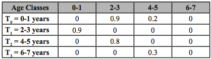
Computation: Using the Leslie Matrix to the right and given an initial abundance of 1000 for age class 2-3, how many individuals will survive to age class 4-5?
| A. |
| B. |
| C. |
| D. |
| E. |
2.
Computation: The dilution factor of 1:20 yields a solution concentration of:
| A. |
| B. |
| C. |
| D. |
| E. |
3.
LOC: Models allow researchers to:
| A. |
| B. |
| C. |
| D. |
| E. |
4.
HOC: Shopon carries out a population experiment on a strain of E. coli bacteria in different media and monitors the growth at 600 nm in a spectrophotometer. Which conclusion is FALSE?
| A. |
| B. |
| C. |
| D. |
| E. |