Chapter 5. LAB 5 MANAGING DATA II : Statistics & Morphology
Learning Goals:
- Know the different types of data
- Know how to determine which statistic to apply to a data set for analysis
- Know the difference between a sample and a population
Lab Outline
Activity 1: Anthropometrics (Prelab)
Activity 2: Working with measurement data from human and stickleback populations
Activity 3: Working with continuous and categorical data from Isopod Behavior experiments
5.1 Scientific Inquiry

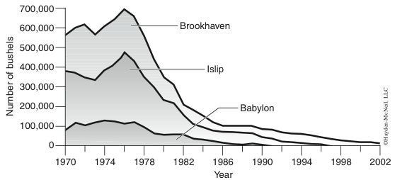
- Why have there been dramatic declines in shell fishery harvests on Long Island (Figure 1)?
- Is there a correlation between shellfish harvest size and overall marine habitat quality?
- How can we restore our ocean resources to the healthy and diverse marine ecosystems they once were?
For a long time, marine resources have been taken for granted and exploited without regard to the consequences of over-fishing and habitat destruction. In the last 25 years, there have been precipitous changes in our marine ecosystems and these changes are reflected in the abundance of our once vital fisheries. How do we distinguish between the changes in animal populations that humans can control vs. changes that are part of “natural cycles” that are not under our control?
Scientists are asked to investigate a huge range of biological issues including ecosystem diversity, health and disease, food production and they seek to develop innovative products and services to address these issues. What are some basic approaches to scientific investigation? How are experiments designed? How are the data produced by these investigations used to draw cause and effect conclusions as well as solutions to our problems?
Science in Action
Conover and Munch, two professors from Stony Brook’s School of Marine and Atmospheric Sciences (SoMAS), have recently contributed answers to these important questions. It is well known that over- fished species have a reduced number of older and larger individuals. It was thought that if only larger fish were taken and smaller individuals and juveniles are spared, that the population would remain relatively undisturbed or rebound easily. Therefore, local, state, and federal governments imposed fishing regulations which restricted the minimum size of many game fish. To test this assumption, Conover and Munch (2002) compared three populations of fish in which 1) only large individuals were removed, 2) only small individuals were removed, and 3) individuals were removed at random.
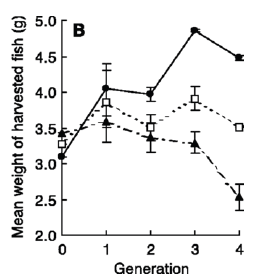
After four generations of this type of selection pressure, an interesting trend emerged—“the mean weight of the harvested individuals from the small-harvested lines was larger than that of the large-harvested lines.” In the small-harvested populations, the individuals who grew fastest as juveniles were more likely to survive whereas in the large-harvested group, individuals that grew most slowly were more likely to survive (Figure 2). Hence, by Generation 4, the mean individual weight at spawning was 1.05g for the large-selected line, and 6.47g for the small-selected line. Does this mean our policies should require us to take only small fish? What happens if we deplete the juveniles who have not yet reproduced?
The authors suggest that effective management plans must consider evolutionary consequences of fishing regulations to preserve natural genetic variation and healthy ecosystem dynamics. “No take zones” and maximum size restrictions (all captured fish must be below a certain size) are two forms of management that might preserve genetic variation in fish so that over-fished populations have the potential to rebound and recover.
5.2 Background
In today’s lab, you will record data from simple measurements of human and fish anatomy. Although this may seem like a trivial exercise, the ability to take measurements that are accurate (as close to the true value as possible) and precise (reproducibility of the measurement) is not as simple as it appears. If ten students measure the length of the same student’s ear lobe even if they use the same instrument (a Vernier caliper), there will be variability in the values due to human measuring error. Thus, if you were measuring two variables to determine if there are significant differences between them, your measurements will include a “real” difference component and an “error” component. Statistics provide standard measures of variability and measurement characteristics to help us identify significant differences.
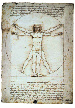
When you think of human body parts, you may think of the Vitruvian Man—the rendition by Leonardo da Vinci of the “proportioned man.” Was Leonardo da Vinci’s drawing meant to illustrate natural relationships between parts of the human body? Or was it a recursive geometrical algorithm meant to approximate the squaring of a circle (a geometric solution to the problem of drawing a circle and a square of equal areas)?
Although the meaning of da Vinci’s Vitruvian man may not interest you, does the field of forensics interest you? How would you determine the height of a suspect from their shoe print? Does shopping for clothes interest you? What information does a clothing manufacturer use to produce properly proportioned clothing for women versus men? Does anthropology interest you? How can you estimate the height of a Neanderthal from the width of their vertebra?
What do all of these questions have in common? Anthropometry: the study of human proportions or body dimensions.
Perhaps you will become a nurse one day What if you need to accurately measure the height of a patient confined to a wheelchair, and they are unable to assume an upright position, even with help. What would you do? Take another look at da Vinci’s drawing. Does it hint at a solution to your problem? Are the outstretched arms of the Vitruvian man the same length as his height? Is this true for you? What about other body parts? Is your hand size proportional to your height? What about the size of your ear? In today’s lab you will collect data to test such hypotheses.
Scientists who study form and shape of living organisms work in a research area known as morphometrics. In morphometrics, geometric equations are used to characterize features and patterns in organism body plans including those that may be dimorphic (i.e., sex-dependent) or ecomorphic (i.e., environment-dependent). Scientists take reproducible measurements of specimens and can use them for their descriptive value and possibly use their analyses to develop phylogenetic hypotheses about the relationships among the specimens. This information can take on further significance if the measured traits are known to have changed over time and the traits are linked to specific genes. Thus morphometrics can be used to link anatomical changes to changes in gene expression.

The three-spined stickleback fish (Gasterosteus aculeatus) is one of many organisms well studied using morphometrics. Three-spined stickleback is a highly variable species that evolves rapidly and exists in a wide range of habitats. It is an extensively researched animal model system and its study allows scientists to make connections between genetics, ecology, evolution, and behavior. These fish can be monitored for evolutionary changes over decades...yes, decades. For example, sticklebacks have a pelvis supported by a pelvic girdle with two pelvic fins attached. There are marine, freshwater, and anadromous populations. In some populations, this pelvic girdle and the fins are reduced or at least much smaller than other populations of sticklebacks. The gene responsible for this reduction is called Pitx1. Scientists have shown that changes in expression of Pitx1 in mice leads to morphological asymmetry—the hind limb on the right side of affected mice are slightly more reduced than the hind limb on their left side (Shapiro et al. 2004). A similar pattern of Pitx1 expression has been found in sticklebacks, the left pelvic spine length was longer than the right.
Three-spined sticklebacks may also have armored plates on their sides. The degree to which armor is present depends on the presence of particular communities of predators in their environment. Stickleback populations that live in lakes where fish and bird predators are prevalent tend to contain a full set (complete morph) of these lateral plates, from 32–36, that stretch from the head to the tail of the fish. In other areas where there are either no predators or insect predators, the plate morph can be medium to low (<9) in number. The variability in plate morphology is dependent on a gene known as Ectodysplasin or EDA (Colosimo et al. 2005).
The stickleback specimens that you will use in today’s lab were collected from Walby Lake and Morvro Lake in Alaska in June 2009 by Dr. Michael Bell of Stony Brook University and former graduate student Dr. Peter Park. The stickleback fish that inhabit these lakes are known as bottom (benthic) feeders. With the exception of Morvro lake populations, in which the lateral plate number is polymorphic (varies considerably within the population), other lakes contain three-spined sticklebacks with low plate numbers. In today’s lab you will use stickleback measurement data to test possible relationships between fish body parts. We will test whether our stickleback population exhibits pelvic spine asymmetry. While you are making your measurements remember that modern scientists can now use a combination of morphometric and molecular genetic information to further our understanding of vertebrate skeletal development and their highly conserved associated genes. Lessons learned from our distant relatives, the fish, are amazingly relevant to mice and other mammals such as humans.
Using statistics to characterize groups of organisms
Scientists are often interested in the degree of correspondence or differences in measured characteristics among groups of organisms. Descriptive statistics such as means and standard deviations are used to characterize a feature of a population that is normally distributed. For example, the entire population of Stony Brook students have an average height called the mean height of the population. If we measure the heights of 25 Stony Brook students, this would be a sample of student heights from this population. But what if the heights were only taken on members of the basketball team? Would that sample be representative of the true population mean? In this case the average heights of Stony Brook students would probably be overestimated because, in general varsity basketball players are quite tall. So if your goal is to determine the mean heights of SBU students, you would want to randomly sample a sufficiently large sample size of the population, so that the mean of your sample is not biased.
However, differences in sample means can be very useful in detecting real differences between groups when there is an underlying cause and effect resulting in measurable differences between groups. For example, mean body length of a species of fish can be used to compare different groups treated with different diets but the experimental design used to compare mean differences in diets is very important.
If one treatment group is composed of larger individuals while another group is composed of smaller individuals before being given the experimental diets, the two groups are not really comparable.
Explain the statement above and discuss what you would do to design an experiment that was unbiased.
5.3 Resources
Bell MA and Foster SA, editors. 1994.The Evolutionary Biology of the Threespine Stickleback. New York: Oxford University Press. 571p.
Colosimo PF, Hosemann KE, Balabhadra S, Guadalupe VJ, Dickson M, Grimwood J, Schmutz J, Myers RM, Schluter D, and Kingsley DM. 2005.Widespread parallel evolution in sticklebacks by repeated fixation of Ectodysplasin alleles. Science 307:1928–1933.
Conover DO and Munch SB. 2002. Sustaining fisheries yields over evolutionary time scales. Science 297: 94 – 96.
Harris M, Taylor G, Taylor J. 2008. Math and Statistics for the Life Sciences. New York: W. H. Freeman.
Knisely K. 2008. A Student Handbook for Writing in Biology, SBU edition. New York:
W. H. Freeman. 221 p.
Reimchen TE and Nosil P. 2001. Lateral plate asymmetry, diet and parasitism in threespine stickleback. Journal of Evolutionary Biology 14:632–645.
Shapiro MD, Marks ME, Peichel CL, Blackman BK, Nereng KS, Jo ́nsson B, Schluter D and Kingsley DM. 2004. Genetic and developmental basis of evolutionary pelvic reduction in threespine sticklebacks. Nature 428: 717–723.
5.4 Lab Preparation

Complete the BioPortal Quiz, which is designed to gauge your understanding of the prerequisites for this course, as well as your knowledge of the required content. It is your responsibility to review this material, if necessary, then watch the vodcast and read this lab. Place all notes in your lab notebook, which can be used during the Pre-Lab Quiz.
5.5 Activity 1: Anthropometrics (Prelab)
Purpose
In this activity you will focus on human body part data collection by proposing a question or possible relationship you want to test. Your group will collect data from a sample size of at least 10 adult individuals (including your group members) on 3 (or more) body dimensions, one of which must be left hand area. You can collect data on any of the listed body dimensions, or dimensions of your choosing if approved by your instructor. We recommended that you collect demographics (sex, age, etc.) for each subject. If you plan to measure parts like fingers, ears, and nose, then Vernier calipers will be most appropriate. You will apply statistics to describe your sample data and use graphical analysis to test for possible correlations between body measurements.
Dimensions (many of these are common anthropometric measurements)

Materials

ImageJ software
Measuring Tape
Ruler
Vernier Caliper
Scanner
5.6 Procedure
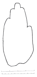
- Hand scan: Trace the left hand of all subjects on a blank white sheet of paper and note their sex, male or female, in the upper right corner of the sheet. The left hand should be traced in a closed conformation with the fingers side-by-side (non-overlapping) using a black superfine marker. You want the line to be dense as shown in Figure 6. White-out any mistakes. Place a ruler nearby and trace two lines, one 4 inches and one 10 centimeters. Mark each inch and each centimeter with a tick mark. Scan each drawing into a computer and save the files in a graphics format such as GIF, TIFF or JPEG on your memory stick. Record the number of pixels per inch at which your hand image was scanned in your lab notebook.
Note: If you have difficulty tracing your hand, copy your hand, and then trace the outline of the copy of the hand with a permanent marker that bleeds through to the other side of the paper. Trace the marks on the opposite side of the paper to produce your hand for scanning. Remember to place the two scales (inches and centimeters) on the paper.
- Hand estimation: Use a ruler to estimate the area of your hand only in inches2 and in centimeters2. Show your calculations and record the area in your lab notebook.
- Additional dimensions: Think like a scientist and devise a well defined method so the additional measurements are taken consistently. Write out your protocol and create a shared (i.e., Google Drive) spreadsheet so that all your group members can input their data.
- ImageJ: Use your scanned images to measure the area of each hand using the ImageJ software. Follow the guide below that shows the tools available in ImageJ.
- Open ImageJ by clicking on the ImageJ icon.
- Go to the “File” menu and click on “Open.” Locate the file of your scanned hand and select it. Your image will open in a separate window. The name of the file will display at the top of the window. Optionally, you can open your hand file by dragging your image file to the icon for ImageJ before you open the program or dragging your image file to the menu bar of ImageJ after you open the program.
- Move the cursor over the scanned image of the hand and notice that the x and y coordinates are displayed in the Status Bar just below the tool bar in the ImageJ window.
- Click on the “line selection tools.” Make sure that the straight line is checked by right clicking on the red ▼ which will display a drop down menu.
- Place the cursor at the first line of your inch ruler and click, while holding down the left mouse button drag the yellow line that appears to the last mark of your ruler and click again to release it. The line will be marked by tiny boxes that span the length of the ruler in your figure (it is best to measure several inches for accuracy).
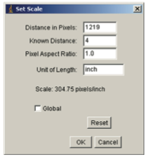
- Set the scale for your measurements by going to the menu bar and choosing Analyze→Set Scale. A menu box will appear. The program will automatically type in the Distance in Pixels for the line you selected. Type the length of your ruler in the space next to Known Distance. Type “in” or “inch” for inches in the space next to Unit of Length. Do not select “Global” unless you have more than one image you wish to measure using the same scale.
- Write down the number of pixels per inch stated for the Scale. Does this match the resolution with which you scanned the image?
- Click OK to complete the setting. Check that your scale is measuring properly as follows. Place the cursor on one end of the ruler and record the coordinate that appears on the status bar (record the x coordinate if you drew your ruler horizontally, and the y coordinate if you drew your ruler vertically). Move the cursor to one inch away from the end of the ruler and record that coordinate. Try it for the next inch on the ruler. Are the values close to one inch? If not, you may need to reset your scale.
- Click the “Wand (tracing) tool” button from the Tool bar.
- Select your entire hand in the image by placing the cursor on the tracing line and left clicking. It will turn yellow to tell you that it is highlighted. If the edge of the page is yellow or if there is one yellow dot on your page, you did not click exactly on the tracing of your hand. Click off of the hand and try again.
- If you experience difficulty with the wand tool, then adjust “thresholding” (binary contrast enhancement). Change the image to 8-bit grayscale: Image→Type→8-bit. To complete the image contrast, select Process→Binary→Make Binary and repeat the use of the wand tool. (You can also opt to use the free hand tool (heart) which requires that you trace the hand as accurately as possible while holding down the mouse button.)
- Go to the menu bar and select Analyze→Measure.
- The Results box will appear on the screen and your hand area will be given in whatever units you entered in the “set scale” screen (inches2 or centimeters2). Record the area.
- Check your value. Is the value calculated by the ImageJ software close to your estimated value? What experiment(s) could you run to test the accuracy of this software in measuring area?
- Repeat the process and measure the hand in square centimeters. You must set the scale using the centimeter ruler and re-measure the area of the hand with the wand tool. Is the value calculated by the ImageJ software close to your estimated value?
- Measure the area for each of the remaining hands in centimeters only. Will you need to reset the centimeter scale for each hand? Explain.
- Prepare a table in Excel similar to table 1. Place all your measurements for your group data into your table. Place your hand area data into the class data sheet separating male hand data from female hand data. You will complete the data analysis for your human body parts anatomy data in class.
- Start collection of your data for Activity 2. You will complete the data analysis for human and stickleback body parts once all the data has been collected.
Table 1 Human Proportions Data

5.7 Activity 2: Working with Measurement Data from Human and Stickleback Populations
Thus far you have worked with human measurement data. In this activity, we will introduce you to three-spined stickleback data collection and then you will proceed to analyze both human and fish data sets and learn when and how to apply different statistical tests.
5.8 Activity 2A: Stickleback Proportions
Purpose
In this activity, each group will analyze sample data from two stickleback populations, one from Walby Lake and one from Morvro Lake. The stickleback measurements (continuous data) include body dimensions of standard length (SL), right and left pelvic spine length (rPLV and lPLV), eye diameter (ED), and caudal peduncle (CP). The number of lateral plates (LPN) for each fish will serve as a categorical data trait. You will use statistics to describe the data, to test for possible relationships between body dimensions, and to test a hypothesis about the asymmetry of right and left pelvic spines. So that you are familiar with how the data you analyze was collected, your group will collect stickleback measurements on one fish from each of the two lakes.
Procedure
Safety: Wear gloves at all times when handling the fish. The fish were fixed using a toxic preservative, rinsed free of preservative, and then stored in isopropyl alcohol. Although there should be undetectable amounts of preservative present on the fish, please exercise proper caution by always handling the fish with gloves. Wear goggles to protect your eyes from splashing alcohol.
- Split your group into two. Retrieve two dissecting microscopes and lamps.
- Prepare a data table similar to Table 2 in your lab notebook. While one person of each pair takes measurements on their specimen, the other will record the data in the Excel spreadsheet. So that all group members can observe the way in which the measurements are taken and view the fish under the microscope, allow the group member who recorded the measurements to count the number of lateral plates on each side of the one fish.
- Position each fish on its side with the head facing your left, the tail towards your right and the ventral side towards you. The side facing up will be the left side of the fish. Take measurements from the left side of each fish for SD, ED, and CP. Refer to the diagram of the three-spined stickleback shown in Figure 4 for a visual description of each type of measurement. Whenever you measure with the calipers, open the caliper jaws wider than needed and slowly close them to the correct length.
- Standard length: Using a ruler, measure the length of the fish from the snout to the caudal vertebra (just anterior to the caudal or tail fin). Record your value in your table.
- Caudle peduncle: Measure the distance from the dorsal to ventral surface of the caudal peduncle using the Vernier caliper. The caudal peduncle is the narrow region where the caudal fin is attached.
- Eye diameter: Measure the length of the eye at its maximal anterior-posterior distances using a Vernier caliper.
- Pelvic Spine Length: You should measure the length of the pelvic spine from the spine socket where the spine joins the body to its distal tip. Flip the fish vertically 180 degrees so that the head is facing your right to measure the right pelvic spine.
- Lateral Plate number: Count the number of plates on each side of the fish.
- Download the data for the variables (SD, ED, CP, lPLV, rPLV, rLPN, and lLPN) from your section course site to begin the data analysis.
How difficult was it to measure the stickleback body dimensions? Do you think that you could design a method to minimize measurement error if you were doing a morphometric-based study on stickleback? Would you have more than one individual collect the data?
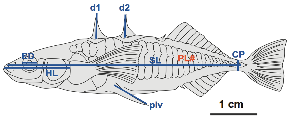
Table 2 Measurements of body parts of three-spined stickleback from __________ Lake

5.9 Activity 2B: Analyzing Data using statistics
Describe your Data
- What techniques will you use to describe your human and stickleback data? Use the Statistics Flowchart on the back cover of your lab notebook. What analysis does it recommend?
- What descriptive characteristics of your data can be calculated using Excel Analysis Toolpak? Your instructor will assist you with this and you should ensure that you understand the type of information that each of these descriptive characters provide and how they might be useful.
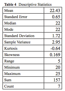
- Determine the mean, mode, median, standard error, and standard deviation of the data separately for each body dimension. The data should look similar to Table 3.
- What is the mean for each of the measurments? How much variability is there for each of the measurements; do certain body parts show more variability than others? If so, why do you think this is?
- As a class, prepare a histogram of the compiled hand area data by both total population sample size and by sex. Histograms and frequency distributions are commonly applied to data to look for trends or patterns. What patterns do you notice when you compare the histograms between male and female hand area size? If you have time at the end of class, make a histogram of your other body dimensions.
Test for possible relationships between your variables
- How would you test whether there are associations between your body dimensions assuming the variables are independent of one another? Dependent on one another? Turn to the back page of your lab notebook to the statistics flowchart. What analysis does it recommend for each of these scenarios? Why does variable independence or dependence matter?
- Use Excel to determine if there is a correlation of hand size with your other body dimensions. For example, if you measured height, is there a positive correlation between hand area and height such that tall people tend to have bigger hands than shorter people.
- Make three scatter plots of pairwise comparisons for your three body dimensions in Excel. Does it matter which variable you place on the x-axis or y-axis for this statistical test?
- Determine the correlation coefficient “R” for each data set using the Excel function for correlation (correl). Based on the “R” values are any of your body dimensions strongly (>0.6) or weakly correlated (<0.4) with each other?
- Can you think of a case in which your data would not support known correlations of body dimensions? Would you expect anatomical correlations for individuals with Marfan Syndrome or dwarfism?
- Use Excel for linear regression analysis. Insert a regression line (trendline) in each of your charts along with the slope equation and “R2” value. How well does the slope equation mathematically map your data? What does the “R2” value tell you about the residual error? For this test it matters what variable you place on the x-axis. This is the independent variable that can predict the value of a dependent variable. If for example you use foot length as your independent variable, you may be able to predict height, your dependent variable. For our purposes, you may arbitrarily select one variable to be the independent variable in each graph.
- Use Excel to determine if ED, SL, or CP show a correlation with each other. Is a stickleback’s body length proportional to its eye diameter? To its caudal peduncle length? Is there a correlation between eye diameter and caudal peduncle size, such that fish with larger CPs also tend to have bigger eyes?
- Make three scatter plots, SL versus CP, SL versus ED, and CP versus ED, in ExcelTM.
- Determine the correlation coefficient “R” value for each of your scatter plots using the Excel function for correlation (correl). Based on the “R” value, are the body parts strongly or weakly correlated with each other?
- Insert a regression line (trendline) in each of your charts along with the slope equation and “R2” value to carry out linear regression analysis. How well does the slope equation describe your data?
Remember: a high correlation suggests a relationship between two variables, but does not determine the cause and effect relationship. For this, you would have to know a great deal more about the nature of these relationships.
5.10 Activity 2C: Comparing Means of sample populations
Purpose
Scientists very commonly compare means (averages) of independent data such as before and after, control and treatment, or changes over time of the same sample for data such as growth. When sample sizes are small, data means can be compared using a common kind of statistical test called a t-test. There are many times when we must make comparisons between means of data in which there is dependence between them—this comparison is called a paired t-test. An example of paired measurements are “before and after exercise” heart rate measurements on the same individual. However, the simplest t-test called an unpaired t-test is used to compare the means of independent samples. An example of independent samples would be average heart rates for two different individuals taken over the same period of time.
We will apply an unpaired t-test to study left-right asymmetry in stickleback pelvic spines and human feet. We are doing the fish fin–human foot comparison because we know that asymmetry in sticklebacks correlate with Pitx1 gene expression and that this gene-specific asymmetry also exists in mouse hindlimbs. This leads to the question: Do asymmetries naturally exist in human populations? We are able to speculate that there are differences between the right and left foot in humans since these body parts are homologous to mouse hindlimbs.
We will use an unpaired t-test to test the hypothesis that there are significant differences in the means for left minus right anatomical asymmetry in human populations and stickleback populations. If we wanted to compare left versus right spine directly or left versus right foot directly, we would not use a t-test because pelvic spine length is dependent on the fish size (SL) just as foot size is dependent on human height. We must compensate for variability that is due solely to this size dependence otherwise our analysis is meaningless—the data may show differences when there really isn’t any, only differences due to organism size. We could do a paired comparison (e.g., rPLV vs. lPLV) using analysis of variance (ANOVA) to gauge whether there might be a significant difference, but this would not take into account the dependence of PLV on SL or dependence of foot length on height. If we include SL or height, we need to do an analysis of covariance (ANCOVA). Because both of these statistics are somewhat complicated for an introductory student, we will look at differences between populations for which unpaired t-tests can be applied.
Refer to the Math Stats Catchup guide for information about this test and the Knisely Appendix for steps on how to use Excel to do the t-test calculations. Make sure you understand the rationale for comparing t-values and determining the critical t-value based on particular significance levels as provided in the Math and Stats Catchup guide.
5.11 Procedure
- For the data provided for each individual population:
- Walby vs. Morvro Lake, subtract the rPLV from the lPLV pelvic spine length data to obtain single values for t-test comparisons.
- Female vs. male foot size, subtract left minus right foot data to obtain single values for t-test comparisons.
- State the hypothesis and the null hypothesis for your two t-test comparisons: the left-right foot data and left-right pelvic spine data.
- What is the null hypothesis for the left-right pelvic spine comparisons for the Morvro and Walby Lakes fish populations? What is the alternate hypothesis?
- The null hypothesis for the right and left human foot by gender comparisons states that there is no significant difference for the mean of the left-right foot data for males versus females. What is the alternate hypothesis?
- Explain why t-test analysis is used for this data. What assumptions must be made to apply the t-test?
- Since we want to compare males versus females within one population (Bio 204 students), a two-tailed unpaired t-test could be used. Should we use a similar statistic for the two different lake populations of sticklebacks?
- Assumption of Normality: Before you proceed with the t-test you need to know if your data is normally distributed? Perform descriptive statistics of your data using ExcelTM then perform a simple check (see Figure 5). If your data (the minimum and the maximum values) lie outside +/- 2 standard deviations (SD) from your mean then it is not normally distributed. (Math and Stats, p.125). Would you expect your stickleback data to be distributed normally?
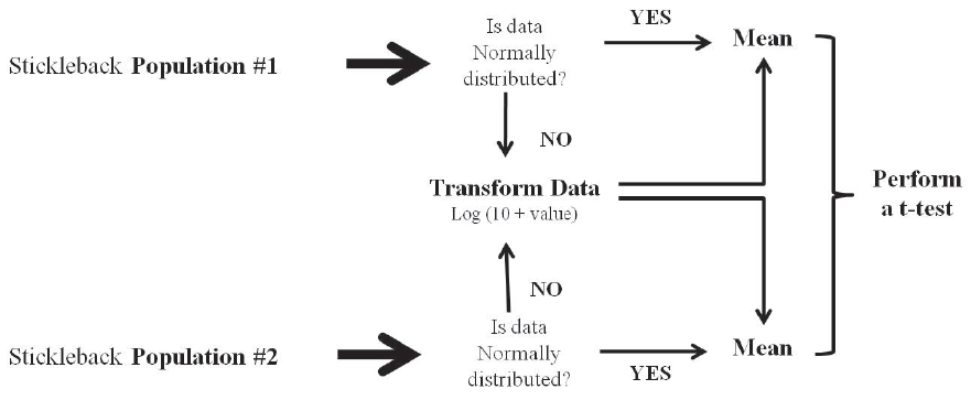
- If the data is skewed, then you need to transform it by adding a constant (e.g. the number 10) and take the log of each value. ExcelTM will automatically do this transformation: type into a cell = log (data value + 10).
- Now we can quickly do the statistical analysis using the Data Analysis Tool Pak in Excel: Data>Data Analysis > “t-test: Two Sample assuming Unequal Variances.” For an example, we will use sample data (Table 4) from an Excel file (only part of the data is displayed) for the L-R foot.
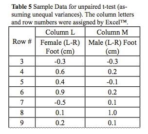
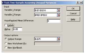
- In the dialog box for the t-test (Figure 6), enter the cell range data for column L as “Variable 1 Range”: $L$3:$L$16 and the cell range data for column M as “Variable 2 Range”: $M$3:$M$12 by first clicking in the box of interest and then highlighting the values in the worksheet.
- What is the “hypothesized mean difference” for the null hypothesis? Place that value in the box.
- Select a cell for the “Output Range” and click OK. Excel will place a table of your analysis in the worksheet positioned at the cell selected for the “Output Range (Table 5).”
- Analyze the output for the stickleback left-right pelvic spine comparison. For an explanation of the parameters in the t-test output table refer to Knisely Appendix. Answer the following questions:
- What conclusion can you draw from your statistical analyses? Is there a difference between the two lake populations with respect to PLV asymmetry?
- Did your t-test results support or reject your null hypothesis? Explain based on your critical t-value.
- Was there much variation for each data set? Explain.
- How strong were the correlations between data sets? Explain.
- The data you received was collected by several individuals. How could this activity be improved to minimize error?
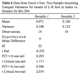
- Analyze output for the human left-right foot comparison. Answer the following questions:
- What conclusion can you draw from your statistical analyses? Is there a difference between the female and male populations with respect to left-right foot asymmetry?
- Did your t-test results support or reject your null hypothesis? Explain based on your critical t-value.
- Was there much variation for each data set? Explain.
- How strong were the correlations between data sets? Explain.
- The data you received was collected by several different individuals. How could the data collection be improved to minimize error?
- Can you make a comparison for any of your body part measurements using a t-test? Explain why or why not.
5.12 Activity 3: Working with continuous and categorical data from Isopod Behavior Experiments

Scientific research involves first making observations, then developing hypotheses (“educated guesses” about phenomena of interest) based on these observations, and finally collecting and analyzing data to test the hypotheses. Good examples of this process often inspire a new set of hypotheses and the cycle continues to develop our understanding of the natural world. One valuable and widely used approach to scientific research (but by no means the only approach) is the use of manipulative experiments. In a manipulative experiment, the researcher varies a specific factor or condition to determine how it affects the phenomenon of interest. This contrasts with the approach of correlation studies, in which the researcher does not control specific factors or conditions, but instead looks at relations between variables as they are found in nature.
In today’s isopod exercise, you will perform a manipulative experiment, monitoring the effects of moisture levels and types on the behavior of this small crustacean. You will test whether the isopods move toward wet (treatment) or dry (control) areas.
Learning Objectives
After successful completion of this activity, you should be able to:
- Use a dissection scope and Vernier caliper
- Formulate a hypothesis and perform basic data analysis
- Measure and compute basic descriptive statistics, ratios, and length measurements
Materials
Isopod arena (8” culture dish with sandpaper bottom)
85W flood light on ring stand
4 sponges
Isopods
RO water
Transfer pipettes
Light meter (or use light meter app)
Vernier caliper
Permanent Marker
Ruler and Vernier calipers
Thermometer, pH meter, and balance
Wear goggles! It is important that you protect your eyes from the potential broken glass. If the flood light is on, wear your goggles.
Purpose
- Write down the question you are asking and the null hypothesis to that question with help from your lab instructor. You will address the concepts of “hypotheses and controls” in more detail in the next lab.
- Obtain four small sponges and measure their LxWxH dimensions with a Vernier caliper. Use a 3 ml transfer pipette to moisten two of the sponges, 3 ml of water on one side of each sponge and 3 ml of water on the other side of each sponge for a total of 6 ml of water. The sponges should be damp throughout. Avoid wetting the other two dry sponges.
- Place the four small sponges around the perimeter of the arena, in alternating order of wet and dry, by leaning the sponges on the walls of the container at the base of the tape on the dishes (these sponges simulate hiding places for the isopods outdoors, such as logs).
- Adjust the 85W incandescent bulb about 20 cm vertically from the center of the arena. Record the temperature of the center of the arena with the light off, turn on the lamp and record the temperature immediately. Your group may want to record the temperature of the center of the arena every minute during your 5 minute experiment.
- Release 20–24 isopods (how many isopods should you have minimally?) into the center of the arena. Record observations of isopod behavior in your lab notebook. You may want to record the number of isopods that are “not” under a sponge after each minute.
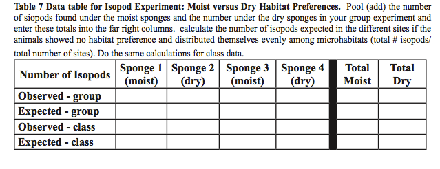
- After 5 minutes, count the number of isopods under each sponge and enter this information into your lab notebook in the format of Table 6.
- Sketch (or photograph) the arrangement and condition (moist or dry) of sponges in the arena.
- Complete the Data Analysis as a class.
5.13 Data Analysis: Chi-square (Goodness of Fit) Test
Background
The isopod behavior experiment can be simplified to one comparison: Are the isopods randomly assorting into categories OR are the isopods distinguishing between the microhabitats and selecting categories based on preference? We will use statistics to determine whether isopods are evenly distributed with respect to the different sites.
Analysis is a Guessing Game without the use of Statistics:
We based our expected counts on the null hypothesis, that the treatment had no effect on isopod behavior thus, isopods should be distributed evenly with respect to the different microhabitats. For example, if there were 20 animals in our arena and 2 possible sites where they could hide, we would expect to find about 10 animals in each site if they showed no preference for the different habitats. However, if the animals display a preference for one site over another, we might observe an uneven distribution of isopods with respect to habitat. But how do we know if this distribution is meaningful and not due to random chance?

If all 20 isopods in the example above were found in one site and 0 were found in the second site, the isopods would be unevenly distributed, and we would conclude that they were displaying a habitat preference. Similarly, if 10 were found in one site and 10 at the second site, the isopods clearly would be evenly distributed, and we would conclude that they had no preference for the two microhabitats offered in the experiment. But what if we found 9 isopods at one site and 11 at another? Would we conclude this to be an equal or an unequal distribution with respect to microhabitat? What about 5 and 15? Do the results differ from the expected results simply due to chance, or due to the treatment effect that we were testing (e.g., wet vs. dry)? Statistics can help us with this question. But what statistical test should we use to analyze our data? Follow this series of questions to determine the right statistical test to select based on our data and experiment.
- What type of question are we asking? Did we compare averages, error, groups, or variables? For our isopod experiments, we studied distributions of isopods, or groups.
- What type of data are we collecting? Did we collect data that was continuous (e.g. length in meters), categorical (e.g. boy & girl), parametric (data are distributed as a bell curve), or circular (measured on a repeating scale; e.g. degrees on a compass)? In today’s lab, our data was the number of isopods under a particular sponge. This is an example of categorical data which is data that can only be certain values or whole numbers. The isopods cannot be split into two and occupy multiple categories at the same time, nor can one isopod occupy a fraction of a category. We will address the other measurements you recorded during this lab after we address the categorical data.
- What type of comparison are we making? Did we compare our sample distribution to one other sample (binomial comparison), to multiple other samples, to a parent distribution, or to a null hypothesis? For this activity we conducted a binomial comparison (wet vs. dry).
- How many comparisons are we making? We are making one comparison between our data and the null hypothesis.
- Are our samples related? Are we independently collecting data or are our samples paired or grouped? The answer is that our data is independently collected. This is why it is important to select new isopods for each trial. If you used the same isopods for two trials, your data from both would be paired. If you used the same isopods over and over, then the samples would be grouped.
- What statistical test(s) should we use based on the answers to the previous questions and the statistics flow chart in your lab notebook? Chi-square or G-test.
Before we use any statistical test to analyze our data, we should always ask the following very important question: What are the assumptions of our statistical test?
Assumptions for Chi-Square:
- Your categorical data must be nominal and not ordinal. An example of ordinal data in which the categories are in order is stages of cancer, where the stages might be 1, 2, 3, etc. An example of nominal data in which the categories are NOT in order is male and female.
- Your sample size must be greater than 5 per category. If it isn’t, this test is inaccurate. This is why it was important to select more than 20 isopods if you used 4 sponges.
Chi-Square Example (also refer to Appendix C and MathStats CatchUp Guide chapter 40): Given the roughly 1:1 ratio of males and females in the human population, we might expect the number of males and females on a bus to be equal at any given time. Suppose we census a bus load of people and find the following:

There seem to be many more females than males on the bus. But, is this deviation from a 1:1 ratio in the number of males to females due to chance or some other cause? To find out, we perform a chi-square test.
Calculating χ2: The general formula for calculating the χ2 statistic is as follows:
χ2 = Σ (observed - expected)2 /expected
For each possible class (in our example there are 2: males or females), you first calculate the difference between the observed and expected values and square this difference. You then divide this squared difference by the expected value, and then sum the values for all possible classes. The larger the difference between the observed and expected values, the larger the χ2 value. In our example:
χ2 = Σ(obs - exp)2 /exp = (30 - 41)2/41 + (52 - 41)2/41 = 2.95 + 2.95 = 5.90
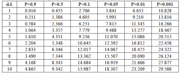
Calculating Probability: The calculated χ2 statistic for these data is 5.90. To determine the probability level (P value) for this test statistic, we first determine the degrees of freedom (d.f.) for the test, then look up the Χ2 value in the probability table (Table 7).
Degrees of Freedom (d.f.): The degrees of freedom are determined by the total number of classes minus 1. Because there are 2 classes in our example (males and females) the degree of freedom is 1 (# of classes - 1 = 2 - 1 = 1 d.f.).
P Values: To determine the probability associated with a given χ2 statistic, look in the row of the table for the appropriate degrees of freedom (in our example d.f.=1, so you look in the first row) and look for your χ2 statistic. You will not find your exact χ2 value, but you can locate which columns, and therefore P values, match your results. If the P value is greater than 5% (to the left of the P=0.05 column), you would conclude that the difference between the observed and expected results is due to chance. If the P value is less than 5% (to the right of the P=0.05 column), then you conclude that the observed distribution is most likely not caused by chance, but rather is caused by some other effect.
Interpreting statistical results: For our bus-rider sample, (χ2=5.90), the number of classes is 2, so d.f.=1 and we look in the first row of the table where 5.90 is found between P=0.05 and P=0.01 (fifth and sixth columns). Thus, the probability that the difference between the observed and expected results is due to chance is very low, between 5% and 1% (0.01 < P <0.05). Because P < 0.05, we can conclude that the greater number of females compared to males on the bus is not due to chance alone, but due to some other effect. In this example, we were not testing a specific treatment effect, so we don’t know the exact cause of the deviation from a 1:1 ratio. However, there may be many possible causes – for example, a Girl Scout Troop might have jumped on the bus just before we took the census.
5.14 Procedure
- Each member of your group should analyze the data from the isopod activity for both group and class data:
- State the specific predictions of the null hypothesis based on the number of isopods used in the experiment.
- Write the equation used to calculate the chi-square value.
- Show the chi-square equation with all of your values entered.
- Show the steps in solving the chi-square equation leading to the final chi-square value.
- State the degrees of freedom (d.f.) used. Show the calculation used to determine d.f.
- Determine the P value from Table 7. You can also calculate the value using Excel (Knisley Appendix).
- Write a few sentences stating the conclusion of your experiment. Compare and contrast your group and class results.
- What additional data did you collect for your experiment? What type of data did you collect? Would you represent this data in tabular or graphical format to learn more about trends in your experiment? Would you apply statistical analyses to any of those data sets? If so, which test(s) and why? What other data could you have collected for this experiment? Explain.
- Turn in your data analysis to your lab instructor.
You will have an opportunity to repeat this study next lab testing your own hypothesis. You should plan to bring in your own supplies if you want to make changes to the isopod arena design (i.e. colored cellophane, filter paper, leaves, bark, etc.). You are welcome to bring in reagents that are innocuous to humans and isopods. It is recommended that you refer to the literature for background on isopods. If you have time at the end of this lab, discuss some questions with your group about isopod behavior that you would like to answer. Be creative with your experimental design.
Table 7 χ2 Test Probability Table
5.15 Self Assessment
These questions were taken from previous exams and are meant to represent a sample, not a complete study guide. The questions in these examples are designed to test your understanding of the concepts and skills presented in this lab, and your ability to apply what you have learned to novel problems.
1.
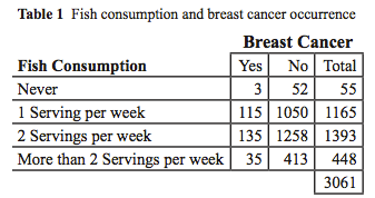
Computation: The table below contains categorical data of a sample of women with and without breast cancer compared with the number of servings of fish that they consume per week. What percent of women surveyed had breast cancer? How many categories would you have if you wanted to do chi square analysis on fish consumption?
2.
LOC: Which of the following is NOT a common morphological landmark used to characterize fish?
| A. |
| B. |
| C. |
| D. |
| E. |
3.
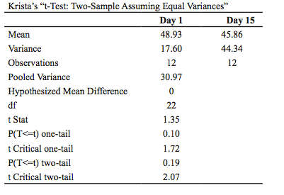
HOC: Krista collects stickleback fish from the same lake on two different days. She compares the difference between the sizes (standard lengths) of the fish based on day. Interpret Krista’s t-test calculation.
| A. |
| B. |
| C. |
| D. |
| E. |
