18.3 Mating Systems
Random mating is a critical assumption of the Hardy–
Assortative mating
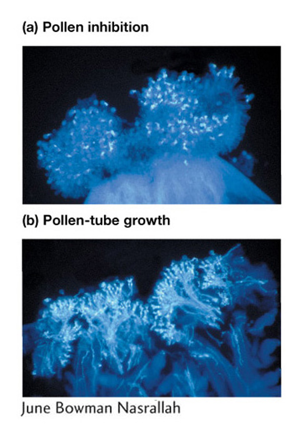
Assortative mating occurs if individuals choose mates based on resemblance to themselves. Positive assortative mating occurs when similar types mate; for example, if tall individuals preferentially mate with other tall individuals and short individuals mate with other short individuals. In these cases, genes controlling the difference in height will not follow the Hardy–
Negative assortative or disassortative mating occurs when unlike individuals mate—
A second example of negative assortative mating is provided by the major histocompatibility complex (MHC), which is known to influence mate choice in vertebrates. MHC affects body odor in mice and rats, providing a basis for mate choice. In what are known as the “sweaty T-
Isolation by distance
Another form of bias in mate choice arises from the amount of geographic distance between individuals. Individuals are more apt to mate with a neighbor than another member of their species on the opposite side of the continent—
If a species has population structure, the proportion of homozygotes will be greater species-
|
Number of individuals |
||||||
|---|---|---|---|---|---|---|
|
N |
A/A |
A/a |
a/a |
p |
q |
|
|
Kansas City |
100 |
81 |
18 |
1 |
0.90 |
0.10 |
|
Hutchinson |
100 |
25 |
50 |
25 |
0.50 |
0.50 |
|
Elkhart |
100 |
1 |
18 |
81 |
0.10 |
0.90 |
|
State- |
300 |
107 |
86 |
107 |
0.50 |
0.50 |
|
State- |
300 |
75 |
150 |
75 |
− |
− |
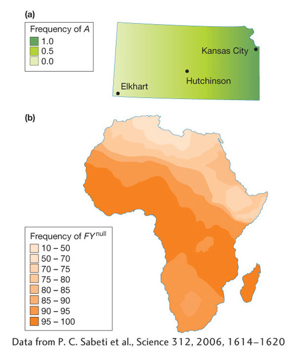
Here is a real example of population structure from our own species. In Africa, the FYnull allele of the Duffy blood group shows a gradient with a low frequency in eastern and northern Africa, moderate frequency in southern Africa, and high frequency across central Africa (Figure 18-11b). This allele is rare outside of Africa. Because of this gradient, we cannot use overall allele frequencies in Africa to calculate genotype frequencies using the Hardy–
KEY CONCEPT
Assortative mating and isolation by distance violate the Hardy–Inbreeding
The third type of bias in mating is inbreeding, or mating between relatives. Long before anyone knew about deleterious recessive alleles, some societies recognized that disorders such as muteness, deafness, and blindness were more frequent among the children of marriages between relatives. Accordingly, brother–
Progeny of inbreeding are more likely to be homozygous at any locus than progeny of non-
The inbreeding coefficient
Inbreeding increases the risk that an individual will be homozygous for a recessive deleterious allele and exhibit a genetic disease. The amount that risk increases depends on two factors: (1) the frequency of the deleterious allele in the population and (2) the degree of inbreeding. To measure the degree of inbreeding, geneticists use the inbreeding coefficient (F), which is the probability that two alleles in an individual trace back to the same copy in a common ancestor. Let’s first consider how to calculate F using pedigrees and then examine how F can be used to determine the increase in risk of inheriting a recessive disease condition.
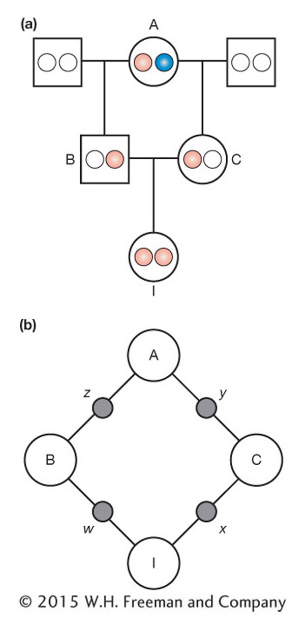
Consider a simple pedigree for a mating between half-
First, since we are only interested in tracing the path of IBD alleles, we can simplify the pedigree to contain only the individuals in the closed loop and still follow the transmission of any IBD alleles (Figure 18-12b). Also, since the sex of the individual doesn’t matter, we use circles for both sexes. The alleles transmitted with each mating are labeled w, x, y, and z. We use “~” to symbolize IBD. We’d like to calculate the probability that w and x are IBD, but let’s take this calculation step by step. First, what is the probability that x and y are IBD or, symbolically, what is P(x ~ y)? This is the probability that C transmits the copy inherited from A to I, which is 1/2, or P(x ~ y) = 1/2. Similarly, the probability that B transmits the copy inherited from A to I is 1/2, or P(w ~ z) = 1/2.
Now we need to calculate the probability that z and y are IBD. There are two ways that z and y can be IBD. The first way is when z and y are both the same copy (both pink or both blue). This happens 1/2 of the time since 1/4 of the time they are both blue and 1/4 both pink. The second way is when z and y are different copies (one pink and the other blue) but individual A was inbred. If individual A is inbred, then there is a probability that her two copies of the gene are IBD. The probability that A’s two copies are IBD is the inbreeding coefficient of A, FA. The probability that z and y are different copies (one pink, the other blue) is 1/2. So, the probability that z and y are different copies that are IBD is 1/2 multiplied by the inbreeding coefficient (FA) to give  FA. Altogether, the probability that z and y are IBD is the probability that they are the same copy (1/2) plus the probability that they are different copies that are IBD (
 FA). Symbolically, we write

P(x ~ y), P(w ~ z), and P(z ~ y) are independent probabilities, so we can use the product rule and put it all together to obtain

In the analysis of inbred pedigrees, we can substitute the value of FA into the equation above if it is known. Otherwise, we can assume FA is zero if there is no information to suggest that individual A is inbred. In the current example, if we assume FA = 0, then

This calculation tells us that the offspring of half-
BOX 18-2 Calculating Inbreeding Coefficients from Pedigrees
In the main text, we saw that the inbreeding coefficient (FI) for the offspring of a mating between half-

where FA is the inbreeding coefficient of the ancestor. This expression includes the term 1/2 to the third power,  . In Figure 18-12, you’ll see there are three individuals in the inbreeding loop, not counting I. The general formula for computing inbreeding coefficients from pedigrees is

where n is the number of individuals in the inbreeding loop not counting I. Let’s look at another pedigree, one in which the grandparents of I are half-
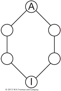
There are five individuals in the inbreeding loop other than I, so if we assume that the ancestor was not inbred (FA = 0), then

In some pedigrees, there is more than one inbreeding loop. Here’s a pedigree in which I is the offspring of a mating between full sibs:
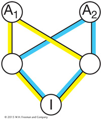
For pedigrees with multiple inbreeding loops, you sum the contribution over all of the loops where FA is the inbreeding coefficient of the ancestor (A) of the given loop:

Thus, for the pedigree where I is the offspring of a mating between full sibs, we get

assuming that the inbreeding coefficients for both ancestors are 0.
When there is inbreeding in a population, the random-

These modified Hardy–
How much does inbreeding increase the risk that offspring will exhibit a recessive disease condition? Table 18-3 shows the inbreeding coefficients for offspring of some different inbred matings and the predicted number of homozygous recessives for different frequencies (q) of the recessive allele. When q = 0.01, there is a 7-
|
Mating |
F |
q = 0.01 |
q = 0.005 |
q = 0.001 |
|---|---|---|---|---|
|
Unrelated parents |
0.0 |
1.00 |
0.25 |
0.01 |
|
Parent- |
1/4 |
25.75 |
12.69 |
2.51 |
|
Half- |
1/8 |
13.38 |
6.47 |
1.26 |
|
First cousin |
1/16 |
7.19 |
3.36 |
0.63 |
|
Second cousin |
1/64 |
2.55 |
1.03 |
0.17 |
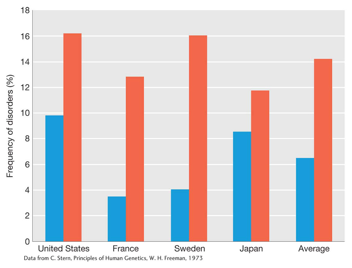
The impact of inbreeding on the frequency of genetic disorders in human populations can be seen in Figure 18-13. Children of marriages of first cousins show about a twofold higher frequency of disorders as compared to children of unrelated parents. Historical records suggest that the risks of inbreeding were understood long before the field of genetics existed.
Population size and inbreeding
Population size is a major factor contributing to the level of inbreeding in populations. In small populations, individuals are more likely to mate with a relative than in large ones. The phenomenon is seen in small human populations such the one on the Tristan de Cunha Islands in the South Atlantic, which has fewer than 300 people. Let’s look at the effect of population size on the overall level of inbreeding in a population as measured by F.
Consider a population with Ft being the level of inbreeding at generation t. To form an individual in the next generation t + 1, we select the first allele from the gene pool. Suppose the population size is N. After the first allele is selected, the probability that the second allele we pick will be exactly the same copy is 1/2N and the inbreeding coefficient for this individual is 1.0. The probability that the second allele we pick will be a different copy from the first allele is 1 − 1/2N and the level of inbreeding for the resulting individual would be Ft, the average inbreeding coefficient for the initial population at generation t. The level of inbreeding in the next generation is the sum of these two possible outcomes or

This equation informs us that F will increase over time as a function of population size. When N is large, F increases slowly over time. When N is small, F increases rapidly over time. For example, suppose Ft in the initial population is 0.1 and N = 10,000. Then Ft+1 would be 0.10005, just a slightly higher value. However, if N = 10, then Ft+1 would be 0.145, a much higher value. We can also use this equation recursively to calculate Ft+2 by using Ft+1 in place of Ft on the right side. The result with N = 10 and Ft = 0.1 would be Ft+2 = 0.188. The effects of population size on inbreeding in populations are further explored in Box 18-
BOX 18-3 Inbreeding in Finite Populations
In the main text, we derived the formula for the increase in inbreeding between generations in finite populations as

which can be rewritten as

We also presented the formula for the frequency of heterozygotes (H) with inbreeding as

which can be rewritten as

Combining these two equations, we obtain

and then

Thus, for each generation, the level of heterozygosity is reduced by the fraction (1 − 1/2N). The reduction in H over t generations is

and the change in F over t generations is given by

As shown in the figure below, inbreeding will increase with time in a finite population even when there is no inbreeding in the initial population.
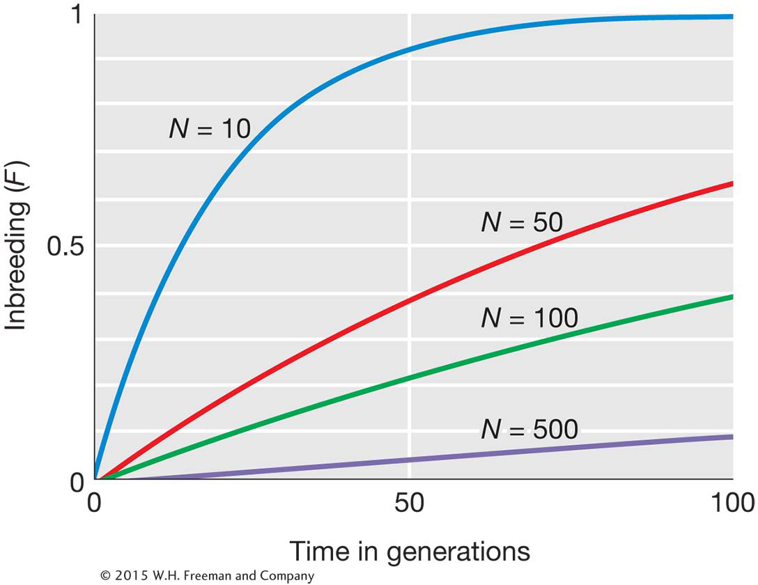
A consequence of the increased inbreeding is that individuals in small populations are more likely to be homozygous for deleterious alleles just as the offspring of first-