19.4 Narrow-Sense Heritability: Predicting Phenotypes
Broad-
The different modes of gene action (interaction among alleles at a locus) are at the heart of understanding narrow-
Gene action and the transmission of genetic variation
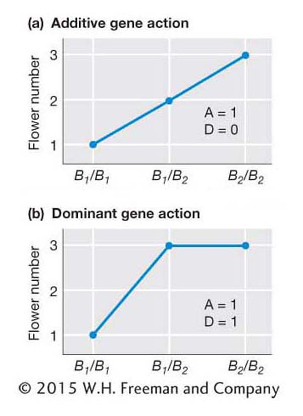
Let’s work through a simple example to show how the mode of gene action influences heritability. Suppose a plant breeder wants to create an improved plant population with more flowers per plant. Flower number is controlled by the B locus, which has two alleles, B1 and B2, as diagrammed in Figure 19-6a. The frequencies of the B1 and B2 alleles are both 0.5, and the frequencies of the B1/B1,B1/B2, and B2/B2 genotypes are 0.25, 0.50, and 0.25, respectively. Plants with the B1/B1 genotype have 1 flower, B1/B2 plants have 2 flowers, and B2/B2 plants have 3 flowers. The mean number of flowers per plant in the population is 2.0. (Remember that we can calculate the mean as the sum of the products of frequency of each class times the value for that class.)
|
Genotype |
Frequency |
Trait value (no. of flowers) |
Contribution to the mean (frequency × value) |
|---|---|---|---|
|
B1/B1 |
0.25 |
1 |
0.25 |
|
B1/B2 |
0.50 |
2 |
1.0 |
|
B2/B2 |
0.25 |
3 |
0.75 |
|
Mean = 2.0 |
Since the heterozygote has a phenotype that is midway between the two homozygous classes, gene action is additive. There are no environmental effects, and the genotype alone determines the number of flowers, so H2 is 1.0. If the plant breeder selects 3-
Now let’s consider the case diagrammed in Figure 19-6b, in which the B2 allele is dominant to the B1. In this case, the B1B2 heterozygote is 3-
|
Genotype |
Frequency |
Phenotype |
Contribution to the mean (frequency × value) |
|---|---|---|---|
|
B1/B2 |
0.25 |
1 |
0.25 |
|
B1/B2 |
0.50 |
3 |
1.5 |
|
B2/B2 |
0.25 |
3 |
0.75 |
|
Mean = 2.5 |
If the plant breeder selects a group of 3-
In conclusion, when there is dominance, we cannot strictly predict the offspring’s phenotypes from the parents’ phenotypes. Some of the differences (variation) among the individuals in the parental generation are due to the dominance interactions between alleles. Since parents transmit their genes but not their genotypes to their offspring, these dominance interactions are not transmitted to the offspring.
The additive and dominance effects
As described above, traits controlled by genes with additive gene action will respond very differently to selection than those with dominance. Thus, geneticists need to quantify the degree of dominance and additivity. In this section, we will see how this is done. Let’s again consider the B locus that controls the number of flowers on a plant (see Figure 19-6). The additive effect (A) provides a measure of the degree of change in the phenotype that occurs with the substitution of one B2 allele for one B1 allele. The additive effect is calculated as the difference between the two homozygous classes divided by 2. For example, as shown in Figure 19-6a, if the trait value of the B1/B1 genotype is 1 and the trait value of the B2/B2 genotype is 3, then

The dominance effect (D) is the deviation of the heterozygote (B1/B2)from the midpoint of the two homozygous classes. As shown in Figure 19-6b, if the trait value of the B1/B1 genotype is 1, of the B1/B2 genotype, 3, and of the B2/B2 genotype, 3, then

If you calculate D for the situation depicted in Figure 19-6a, you’ll find D = 0; that is, no dominance.
The ratio of D/A provides a measure of the degree of dominance. For Figure 19-6a, D/A = 0.0, indicating pure additivity or no dominance. For Figure 19-6b, D/A = 1.0, indicating complete dominance. A D/A ratio of −1 would indicate a complete recessive. (The distinction between dominance and recessivity depends on how the phenotypes are coded and is in this sense arbitrary.) Values that are greater than 0 and less than 1 represent partial dominance, and values that are less than 0 and greater than −1 represent partial recessivity.
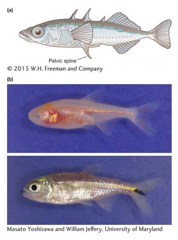
Here is an example of calculating additive and dominance effects at a single locus. Three-
Pitx1 is one of several genes that contributes to pelvic-
|
s/s |
s/l |
l/l |
|---|---|---|
|
0.068 |
0.132 |
0.148 |
Using these values and the formulas above, we can calculate the additive and dominance effects. The additive effect (A) is
(0.148 – 0.068)/2 = 0.04
or 4 percent of body length. The dominance effect (D) is
0.132 – [(0.148 + 0.068)/2] = 0.024
The dominance/additivity ratio is
0.024/0.04 = 0.6
The 0.6 value for the ratio indicates that the long (l) allele of Pitx1 is partially dominant to the short (s) allele.
One can also calculate additive and dominance effects averaged over all the genes in the genome that affect the trait. Here is an example using cave fish (Astyanax mexicanus) and their surface relatives (Figure 19-7b). The cave populations have highly reduced (small-
Horst Wilkins at the University of Hamburg measured mean eye diameter (in mm) for the cave and surface populations and their F1 hybrid:
|
Cave |
F1 |
Surface |
|---|---|---|
|
2.10 |
5.09 |
7.05 |
Using the formulas above, we calculate that A = 2.48, D = 0.52, and D/A = 0.21. In this case, gene action is closer to a purely additive state, although the surface genome is slightly dominant.
KEY CONCEPT
When the trait value for the heterozygous class is midway between the two homozygous classes, gene action is called additive. Any deviation of the heterozygote from the midpoint between the two homozygous classes indicates a degree of dominance of one allele. The additive (A) and dominance (D) effects and their ratio (D/A) provide metrics for quantifying the mode of gene action.A model with additivity and dominance
The example above with the B locus and flower number shows that we cannot accurately predict offspring phenotypes from parental phenotypes when there is dominance, although we can do so in cases of pure additivity. When predicting the phenotypes of offspring, we need to separate the additive and dominance contributions. To do this, we need to modify the simple model introduced in Section 19.2, x = g + e.
Let’s begin by looking more closely at the situation depicted in Figure 19-6b. Individuals with the B1/B2 and B2/B2 genotypes have the same phenotype, 3 flowers. If we subtract the population mean (2.5) from their trait value (3), we see that they have the same genotypic deviation (g):

Now let’s calculate the mean phenotypes of their offspring. If we self- B1/B1,
 B1/B2, and
  B2/B2, and the mean trait value of these offspring would be 2.75. However, if we self-
We can expand the simple model (x = g + e) to incorporate the additive and dominance contributions. The genotypic deviation (g) is the sum of two components—

The additive deviation is transmitted from parent to offspring in a predictable way. The dominance deviation is not transmitted from parent to offspring since new genotypes and thus new interactions between alleles are created each generation.
Let’s look at how the genetic deviation is decomposed into the additive and dominance deviations for the case shown in Figure 19-6b.
|
B1B1 |
B1B2 |
B2B2 |
|
|---|---|---|---|
|
Trait value |
1 |
3 |
3 |
|
Genetic deviation (g) |
−1.5 |
0.5 |
0.5 |
|
Additive deviation (a) |
−1 |
0 |
1 |
|
Dominance deviation (d) |
−0.5 |
0.5 |
−0.5 |
The genotypic deviations (g) are simply calculated by subtracting the population mean (2.5) from the trait value for each genotype. Each genotypic deviation is then decomposed into the additive (a) and dominance (d) deviations using formulas that are beyond the scope of this book. These formulas include the additive (A) and dominance (D) effects as well as the frequencies of the B1 and B2 allele in the population. You’ll notice that a + d sum to g. The additive (a) and dominance (d) deviations are dependent on the allele frequencies because the phenotype of an offspring receiving a B1 allele from one parent will depend on whether that allele combines with a B1 or B2 allele from the other parent, and that outcome depends on the frequencies of the alleles in the population.
The additive deviation (a) has an important meaning in plant and animal breeding. It is the breeding value, or the part of an individual’s deviation from the population mean that is due to additive effects. This is the part that is transmitted to its progeny. Thus, if we wanted to increase the number of flowers per plant in the population, the B2/B2 individuals have the highest breeding value. Breeding values can also be calculated for the genome overall for an individual. Animal breeders estimate the genomic breeding values of individual animals, and these estimates can determine the economic value of the animal.
We have partitioned the genetic deviation (g) into the additive (a) and dominance (d) deviations. Using algebra similar to that described in Box 19-2, we can also partition the genetic variance into the additive and dominance variances as follows:
Vg = Va + Vd
where Va is the additive genetic variance and Vd is the dominance variance. Va is the variance of the additive deviations or the variance of the breeding values. It is the part of the genetic variation that is transmitted from parents to their offspring. Vd is the variance of the dominance deviations. Finally, we can substitute these terms in the equation for the phenotypic variance presented earlier in the chapter:

where Ve is the environmental variance. This equation assumes that the additive and dominance components are not correlated with the environmental effects. This assumption will be true in experiments in which individuals are randomly assigned to environments.
Thus far, we have described models with genetic, environmental, additive, and dominance deviations and variances. In quantitative genetics, the models can get even more complex. In particular, the models can be expanded to include interaction between factors. If one factor alters the effect of another factor, then there is an interaction. Box 19-
BOX 19-4 Interaction Effects
The simple model for decomposing traits into genetic and environmental deviations, x = g + e, assumes that there is no genotype-
If there is no interaction, then the difference in trait value between the inbred lines will be the same in both environments, as shown by the graph on the left.
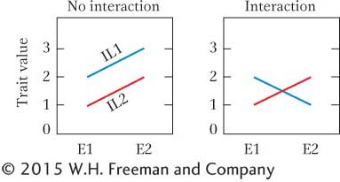
With no interaction, the difference between the two inbreds is 1.0 in both environments, and so the difference between the lines averaged over the two environments is 1.0.
Environment 1: IL1 – IL2 = 2 – 1 = 1.0
Environment 2: IL1 – IL2 = 3 – 2 = 1.0
The difference in the overall mean shows that the lines are genetically different. The mean over both environments is 2.5 for IL1 and 1.5 for IL2.
The graph on the right shows a case of an interaction between genotype and environment. IL1 does well in Environment 1 but poorly in Environment 2. The opposite is true for IL2. The difference in the trait value between the two lines is +1.0 in Environment 1 but – 1.0 in Environment 2.
Environment 1: IL1 – IL2 = 2 – 1 = +1.0
Environment 2: IL1 – IL2 = 1 – 2 = −1.0
The difference between the lines averaged over the two environments is 0.0, so we might incorrectly conclude that these inbreds are genetically equivalent if we looked just at the overall mean.
The simple model can be expanded to include a genotype-
x = g + e + g × e
and
VX = Vg + Ve + Vg × e
where Vg × e is the variance of the genotype-
Interactions can also occur between the alleles at separate genes. This type of interaction is called epistasis. Let’s look at how epistatic interactions affect variation in quantitative traits.
Consider two genes, A with alleles A1 and A2 and B with alleles B1 and B2. The left side of the table below shows the case of no interaction between these genes. Starting with the A1/A1; B1/B1 genotype, whenever you substitute an A2 allele for an A1 allele, the trait value goes up by 1 regardless of the genotype at the B locus. The same is true when substituting alleles at the B locus. The effects of alleles at the A locus are independent of those at the B locus and vice versa. There is no interaction or epistasis.
|
No interaction |
Interaction |
|||||||
|---|---|---|---|---|---|---|---|---|
|
B1/B1 |
B1/B2 |
B2/B2 |
B1/B1 |
B1/B2 |
B2/B2 |
|||
|
A1/A1 |
0 |
1 |
2 |
A1/A1 |
0 |
1 |
2 |
|
|
A1/A2 |
1 |
2 |
3 |
A1/A2 |
0 |
1 |
3 |
|
|
A2/A2 |
2 |
3 |
4 |
|
A2/A2 |
0 |
1 |
4 |
Now look at the right side of the table. Starting with the A1/A1; B1/B1 genotype, substituting an A2 allele for an A1 allele only has an effect on the trait value when the genotype at the B locus is B2/B2. The effects of alleles at the A locus are dependent of those at the B locus. There is an interaction or epistasis between the genes.
The genetic model can be expanded to include an epistatic or interaction term (i):
x = a + d + i + e
and
VX = Va + Vd + Vi + Ve
where Vi is the interaction or epistatic variance.
If the interaction term is not included in the model, then there is an implicit assumption that the genes work independently; that is, there is no epistasis. The interaction variance (Vi), like the dominance variance, is not transmitted from parents to their offspring since new genotypes and thus new epistatic relationships are formed with each generation.
KEY CONCEPT
The genetic deviation (g) of an individual from the population mean is composed of two parts—The genetic variation for a trait in a population (Vg) can be decomposed into the additive (Va) and the dominance (Vd) variances. The additive variance is the fraction of the genetic variation that is transmitted from parent to offspring.
Narrow-sense heritability
We can now define narrow-

This form of heritability measures the extent to which variation among individuals in a population is predictably transmitted to their offspring. Narrow-
To estimate h2, we need to measure Va, but how can this be accomplished? Using algebra and logic similar to that we used to show that Vg can be estimated using the covariance between monozygotic twins reared separately (see Box 19-3), it can also be shown that the covariance between a parent and its offspring is equal to one-

The parent-

To estimate Va using the covariance between parents and offspring requires controlling environmental factors in experiments. This can be a challenge because parents and offspring are necessarily reared at different times. Va can also be estimated using the covariance between half-
If you compare the equation for h2 to the one for H2 (see Box 19-3), you will see that both involve the ratio of a covariance to a variance. The correlation coefficient introduced earlier in the chapter is also the ratio of a covariance to a variance. We are using the degree of correlation among relatives to infer the extent to which traits are heritable.
Here is an exercise that your class can try. Have each student submit his or her height and the height of their same-
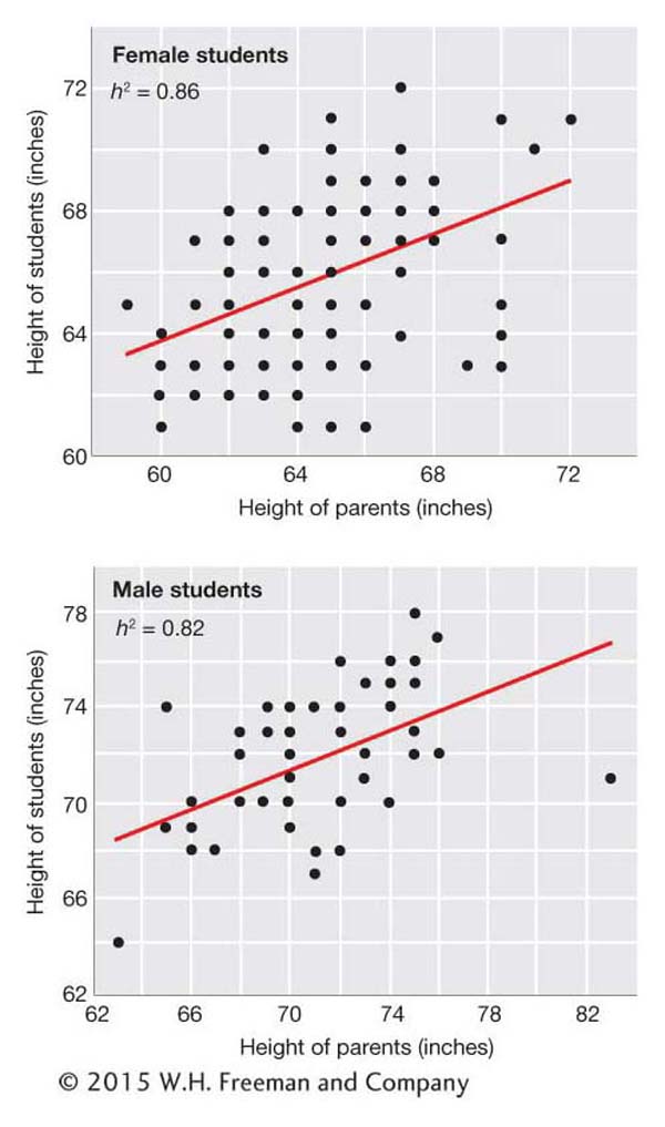
Typically, values for narrow-
Figure 19-8 is a scatter plot with the height data for male and female students and their parents. There is a clear correlation between the heights of the students and their same-
Here are a few more points about narrow-
Narrow-
|
Trait |
h2 (%) |
|---|---|
|
Agronomic species |
|
|
Body weight in cattle |
65 |
|
Milk yield in cattle |
35 |
|
Back- |
70 |
|
Litter size in pig |
5 |
|
Body weight in chicken |
55 |
|
Egg weight in chicken |
50 |
|
Natural species |
|
|
Bill length in Darwin’s finch |
65 |
|
Flight duration in milkweed bug |
20 |
|
Plant height in jewelweed |
8 |
|
Fecundity in red deer |
46 |
|
Life span in collared flycatchers |
15 |
|
Source: D. F. Falconer and T. F. C. Mackay, Introduction to Quantitative Genetics, Longman, 1996; J. C. Conner and D. L. Hartl, A Primer in Ecological Genetics, Sinauer, 2004. |
|
Predicting offspring phenotypes
In order to efficiently improve crops and livestock for traits of agronomic importance, the breeder must be able to predict an offspring’s phenotype from its parents’ phenotypes. Such predictions are made using the breeder’s knowledge of narrow-
x = a + d + e
The additive part is the heritable part that is transmitted to the offspring. Let’s look at a set of parents with phenotypic deviations x′ for the mother and x″ for the father. The parents’ dominance deviations (d′ and d″) are not transmitted to their offspring since new genotypes and new dominance interactions are created with each generation. Similarly, the parents do not transmit their environmental deviations (e′ and e″) to their offspring.
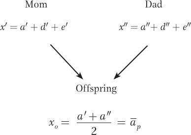
Thus, the only factors that parents transmit to their offspring are their additive deviations (a′ and a″). Accordingly, we can estimate the offspring’s phenotypic deviation (xo) as the mean of the additive deviations of its parents ( ).
).
So to predict the offspring’s phenotype, we need to know its parents’ additive deviations. We cannot directly observe the parents’ additive deviations, but we can estimate them. The additive deviation of an individual is the heritable part of its phenotypic deviation; that is,

where  signifies an estimate of the additive deviation or breeding value. Thus, we can estimate the mean of the parents’ additive deviations as the product of h2 times the mean of their phenotypic deviation and this product will be an estimate of the phenotypic deviation of the offspring (
 ):
):

or

The offspring will have its own dominance and environmental deviations. However, these cannot be predicted. Since they are deviations, they will be zero on average over a large number of offspring.
Here is an example. Icelandic sheep are prized for the quality of their fleece. The average adult sheep in a particular population produces 6 lb of fleece per year. A sire that produces 6.5 lb per year is mated with a dam that produces 7.0 lb per year. The narrow-

Now multiply h2 times  to determine
  , the estimated phenotypic deviation of the offspring:
0.4 × 0.75 = 0.3
Finally, add the population mean (6.0) to the predicted phenotypic deviation of the offspring (0.3) and obtain the result that the predicted phenotype of the offspring is 6.3 lb of fleece per year.
It may seem surprising that the offspring are predicted to produce less fleece than either parent. However, this outcome is expected for a trait with a modest heritability of 0.4. Most (60 percent) of the superior performance of the parents is due to dominance and environmental factors that are not transmitted to the offspring. If the heritability were 1.0, then the predicted value for the offspring would be midway between the parents’. If the heritability were 0.0, then the predicted value for the offspring would be at the population mean since all the variation would be due to nonheritable factors.
Selection on complex traits
Our final topic regarding narrow-
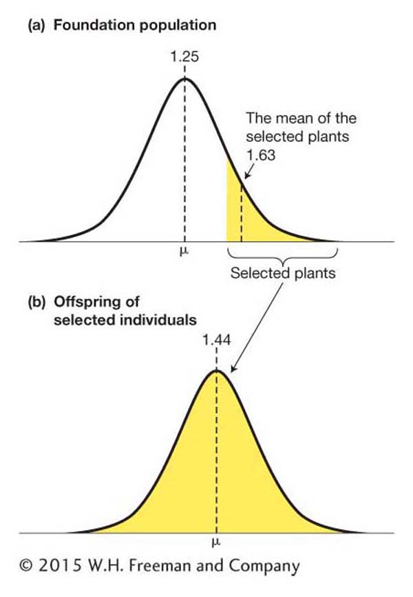
Selection is a process by which only individuals with certain features contribute to the gene pool that forms the next generation (see Chapters 18 and 20). Selection applied by humans to improve a crop or livestock population is termed artificial selection to distinguish it from natural selection. Let’s look at an example of how artificial selection works.
Provitamin A is a precursor in the biosynthesis of vitamin A, an important nutrient for healthy eyes and a well-
If the narrow-

and rewrite it as

 is the mean deviation of the parents (the selected plants) from the population mean. This is known as the selection differential (S), the difference between the mean of the selected group and that of the base population. For our example,

 is the mean deviation of the offspring from the population mean. This is known as the selection response (R), the difference between the mean of the offspring and that of the base population. For our example,

Now we can calculate the narrow-

The underlying logic of this calculation is that the response represents the heritable or additive part of the selection differential.
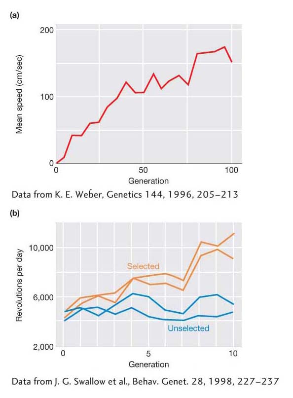
Over the last century, quantitative geneticists have conducted a large number of selection experiments like this. Typically, these experiments are performed over many generations and are referred to as long-
Here are two examples of long-