Example 5.21

EXAMPLE 5.21

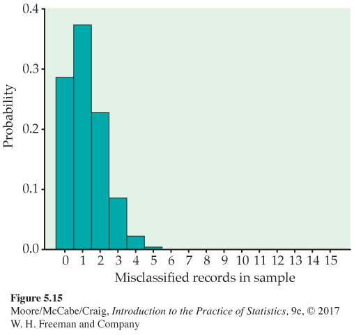
The probability histogram. Suppose that the audit in Example 5.19 chose just 15 sales records. What is the probability that no more than one of the 15 is misclassified? The count X of misclassified records in the sample has approximately the B(15, 0.08) distribution. Figure 5.15 is a probability histogram for this distribution. The distribution is strongly skewed. Although X can take any whole-number value from 0 to 15, the probabilities of values larger than 5 are so small that they do not appear in the histogram.

Figure 5.15 Probability histogram for the binomial distribution with n = 15 and p = 0.08, Example 5.21.

We want to calculate

		p
n	k	.08
15	0	.2863
	1	.3734
	2	.2273
	3	.0857
	4	.0223
	5	.0043
	6	.0006
	7	.0001
	8
	9

P(X ≤ 1) = P(X = 0) + P(X = 1)

when X has the B(15, 0.08) distribution. To use Table C for this calculation, look opposite n = 15 and under p = 0.08. The entries in the rows for each k are P(X = k). Blank cells in the table are 0 to four decimal places. You see that

P(X ≤ 1) = P(X = 0) + P(X = 1)

= 0.2863 + 0.3734 = 0.6597

About two-thirds of all samples will contain no more than one bad record. In fact, almost 29% of the samples will contain no bad records. The sample of size 15 cannot be trusted to provide adequate evidence about misclassified sales records. A larger number of observations is needed.