Example 5.3

EXAMPLE 5.3

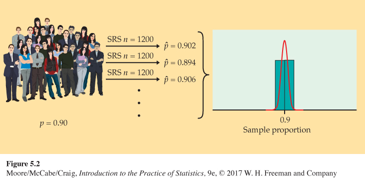
Take many random samples. Figure 5.1 illustrates the process of choosing many samples and finding the statistic for each one. Follow the flow of the figure from the population at the left, to choosing an SRS and finding the for this sample, to collecting together the ’s from many samples. The histogram at the right of the figure shows the distribution of the values of from 1000 separate SRSs of size 100 drawn from a population with p = 0.9.

histogram, p. 14

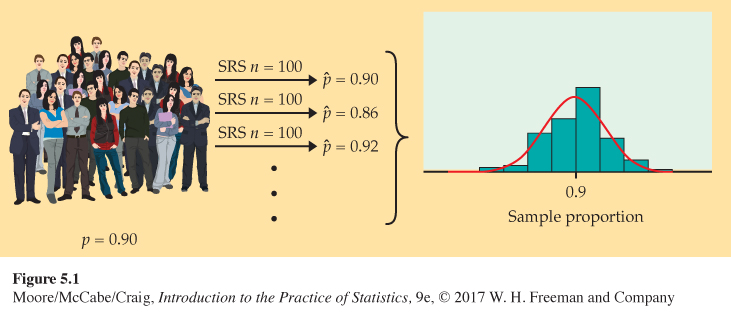
Figure 5.1 The results of many SRSs have a regular pattern, Example 5.3. Here we draw 1000 SRSs of size 100 from the same population. The population parameter is p = 0.9. The histogram shows the distribution of 1000 sample proportions.

Of course, Student Monitor samples 1200 students, not just 100. Figure 5.2 is parallel to Figure 5.1. It shows the process of choosing 1000 SRSs, each of size 1200, from a population in which the true proportion is p = 0.9. The 1000 values of from these samples form the histogram at the right of the figure. Figure 5.1 and 5.2 are drawn on the same scale. Comparing them shows what happens when we increase the size of our samples from 100 to 1200. These histograms display the sampling distribution of the statistic for two sample sizes.

Figure 5.2 The distribution of the sample proportion for 1000 SRSs of size 1200 drawn from the same population as in Figure 5.1. The two histograms have the same scale. The statistic from the larger sample is less variable.