EXAMPLE 7.12
Computing an approximate 95% confidence interval for the difference in means. First examine the data:
| Control | Treatment | |
| 970 | 1 | |
| 860 | 2 | 4 |
| 773 | 3 | 3 |
| 8632221 | 4 | 3334699 |
| 5543 | 5 | 23467789 |
| 20 | 6 | 127 |
| 7 | 1 | |
| 5 | 8 |
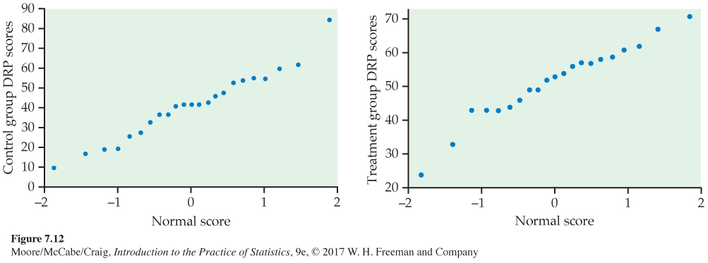
The back-to-back stemplot suggests that there is a mild outlier in the control group but no deviation from Normality serious enough to forbid use of t procedures. Separate Normal quantile plots for both groups (Figure 7.12) confirm that both distributions are approximately Normal. The scores of the treatment group appear to be somewhat higher than those of the control group. The summary statistics are
Page 439
| Group | n | ˉx | s |
|---|---|---|---|
| Treatment | 21 | 51.48 | 11.01 |
| Control | 23 | 41.52 | 17.15 |
To describe the size of the treatment effect, let’s construct a confidence interval for the difference between the treatment group and the control group means. The interval is
(ˉx1-ˉx2)±t*√s21n1+s22n2=(51.48-41.52)±t*√11.01221+17.15223
= 9.96 ± 4.31t*
| df = 20 | |||
| t* | 1.725 | 2.086 | 2.197 |
| C | 0.90 | 0.95 | 0.96 |
The second degrees of freedom approximation uses the t(20) distribution.
Table D gives t* = 2.086. With this approximation, we have
9.96 ± (4.31 × 2.086) = 9.96 ± 8.99 = (1.0, 18.9)
We estimate the mean improvement to be about 10 points, with a margin of error of almost 9 points. Unfortunately, the data do not allow a very precise estimate of the size of the average improvement.