EXAMPLE 7.7
The effect of altering a software parameter. The MeasureMind® 3D MultiSensor metrology software is used by various companies to measure complex machine parts. As part of a technical review of the software, researchers at GE Healthcare discovered that unchecking one software option reduced measurement time by 10%. This time reduction would help the company’s productivity provided the option has no impact on the measurement outcome. To investigate this, the researchers measured 51 parts using the software both with and without this option checked.3 The experimenters tossed a fair coin to decide which measurement (with or without the option) to take first.
Table 7.2 gives the measurements (in microns) for the first 20 parts. For analysis, we subtract the measurement with the option on from the measurement with the option off. These differences form a single sample and appear in the “Diff” columns for each part.
| Part | OptionOn | OptionOff | Diff | Part | OptionOn | OptionOff | Diff |
|---|---|---|---|---|---|---|---|
| 1 | 118.63 | 119.01 | 0.38 | 11 | 119.03 | 118.66 | −0.37 |
| 2 | 117.34 | 118.51 | 1.17 | 12 | 118.74 | 118.88 | 0.14 |
| 3 | 119.30 | 119.50 | 0.20 | 13 | 117.96 | 118.23 | 0.27 |
| 4 | 119.46 | 118.65 | −0.81 | 14 | 118.40 | 118.96 | 0.56 |
| 5 | 118.12 | 118.06 | −0.06 | 15 | 118.06 | 118.28 | 0.22 |
| 6 | 117.78 | 118.04 | 0.26 | 16 | 118.69 | 117.46 | −1.23 |
| 7 | 119.29 | 119.25 | −0.04 | 17 | 118.20 | 118.25 | 0.05 |
| 8 | 120.26 | 118.84 | −1.42 | 18 | 119.54 | 120.26 | 0.72 |
| 9 | 118.42 | 117.78 | −0.64 | 19 | 118.28 | 120.26 | 1.98 |
| 10 | 119.49 | 119.66 | 0.17 | 20 | 119.13 | 119.15 | 0.02 |
Page 420
To assess whether there is a difference between the measurements with and without this option, we test
H0: μ = 0
Ha: μ ≠ 0
Here, μ is the mean difference for the entire population of parts. The null hypothesis says that there is no difference, and Ha says that there is a difference, but does not specify a direction.
The 51 differences have
ˉx = 0.0504 and s = 0.6943
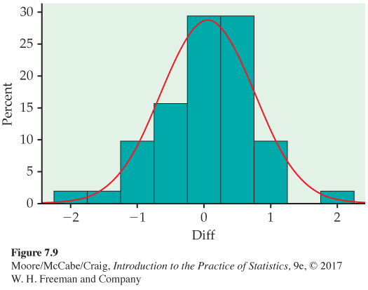
Figure 7.9 shows a histogram of the differences. It is reasonably symmetric with no outliers, so we can comfortably use the one-sample t procedures. Remember to always check assumptions before proceeding with statistical inference.
The one-sample t statistic is
t=ˉx−0s/√n=0.05040.6943/√51
= 0.52
The P-value is found from the t(50) distribution. Remember that the degrees of freedom are 1 less than the sample size.
Table D shows that 0.52 lies to the left of the first column entry. This means the P-value is greater than 2(0.25) = 0.50. Software gives the exact value P = 0.6054. There is little evidence to suggest this option has an impact on the measurements. When reporting results, it is usual to omit the details of routine statistical procedures; our test would be reported in the form: “The difference in measurements was not statistically significant (t = 0.52, df = 50, P = 0.61).”