SECTION 10.1 EXERCISES
For Exercise 10.1, see page 560; for Exercise 10.2, see page 565; for Exercises 10.3 and 10.4, see page 570; for Exercises 10.5 and 10.6, see pages 573–
Question 10.7
10.7 What’s wrong? For each of the following, explain what is wrong and why.
(a) The parameters of the simple linear regression model are b0, b1, and s.
(b) To test H0: b1 = 0, use a t test.
(c) For a particular value of the explanatory variable x, the confidence interval for the mean response will be wider than the prediction interval for a future observation.
10.7 (a) The parameters of the regression model are β0, β1, and ϵ; those given are estimates of these. (b) It should be H0: β1 = 0. (c) The prediction interval will be wider than the mean response interval.
Question 10.8
10.8 What’s wrong? For each of the following, explain what is wrong and why.
(a) The slope describes the change in x for a change in y.
(b) The population regression line is y = b0 + b1x.
(c) A 95% confidence interval for the mean response is the same width regardless of x.
Question 10.9
![]() 10.9 Importance of Normal model deviations. A general form of the central limit theorem tells us that the sampling distributions of b0 and b1 will be approximately Normal even if the model deviations are not Normally distributed. Using this fact, explain why the Normal distribution assumption is much more important for a prediction interval than for the confidence interval of the mean response at x = x*.
10.9 Importance of Normal model deviations. A general form of the central limit theorem tells us that the sampling distributions of b0 and b1 will be approximately Normal even if the model deviations are not Normally distributed. Using this fact, explain why the Normal distribution assumption is much more important for a prediction interval than for the confidence interval of the mean response at x = x*.
10.9 Prediction intervals concern individuals instead of means. Departures from the Normal distribution assumption would be more severe here.
Question 10.10
10.10 Complete check of the residuals. In Example 10.12 (page 574), we checked model assumptions using a scatterplot (Figure 10.9). Let’s consider assessing the model assumptions using the residuals.
(a) Fit the (EDUC, INC) data using least-
squares regression and obtain the residuals. Write down the least- squares regression line .(b) Generate a plot of the residuals versus EDUC and comment on the pattern. Does a linear fit appear reasonable? Does there appear to be constant variance? Are there any unusual observations? Explain your answers.
(c) Construct a histogram and a Normal quantile plot of the residuals. Do the residuals appear Normal? Explain your answer.
(d) Analysis of the residuals is typically done because patterns in the residuals are easier to see. Do you think the plots in parts (b) and (c) magnify the violations of assumptions better than the scatterplot in Figure 10.9? Write a short paragraph comparing the scatterplot with the residual plots.
Question 10.11
10.11 Complete check of the residuals, continued. Refer to the previous exercise. In Example 10.13 (page 575), we checked model assumptions using a scatterplot (Figure 10.10) after log transforming the response variable.
(a) Repeat parts (a) through (c) of the previous exercise using LOGINC and EDUC.
(b) Do you think we can comfortably perform inference using the log transformed y? Explain your answer.
10.11 (a) ˆy = 8.25464 + 0.11259EDUC. The points in the residual plot look scattered and random so the assumptions are satisfied. The histogram shows the residuals are Normally distributed. (b) Yes, the log transformed data can effectively be used for inference.
Question 10.12
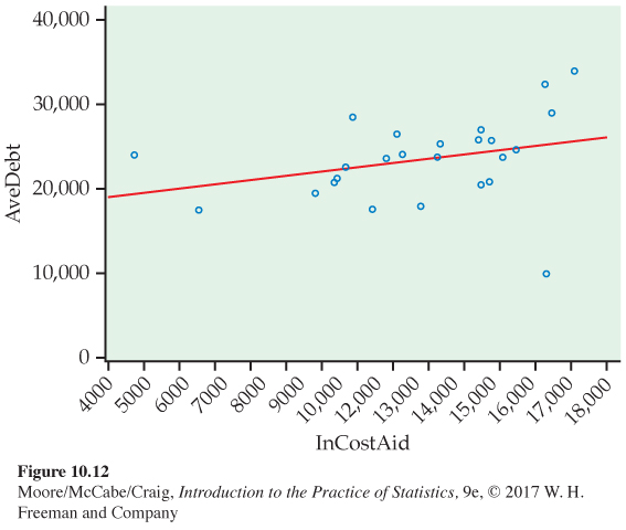
10.12 College debt versus adjusted in-
(a) Does a linear relationship between InCostAid and AveDebt seem reasonable? Explain your answer.
(b) Are there any unusual cases in this sample? If yes, state which ones they are and how they may be affecting the least-
squares model fit.
Question 10.13
10.13 Can we consider this an SRS? Refer to the previous exercise. The report states that Kiplinger’s rankings focus on traditional four-
10.13 Because the list was narrowed before we took our SRS, our sample really only reflects the schools that met the “academic quality” criteria and not all 500 + colleges.
Question 10.14
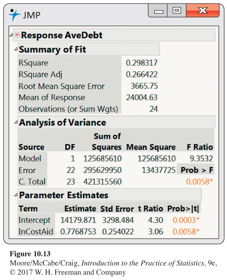
10.14 Predicting college debt. Refer to Exercise 10.12. Baruch College has substantially less average debt compared to the other schools with similar in-
(a) State the least-
squares regression line. (b) The University of North Florida is one school in this sample. It has an in-
state cost of $11,421 and average debt of $17,617. What is the residual? (c) Construct a 95% confidence interval for the slope. What does this interval tell you about the change in average debt for a $1000 change in the in-
state cost? (d) Penn State University is reported to have an adjusted in-
state cost of $23,053. Discuss the appropriateness of using this data set to predict the average debt for this university.
Question 10.15
10.15 More on predicting college debt. Refer to the previous exercise. Appalachian State University has an in-
(a) Using your answer to part (a) of the previous exercise, what is the predicted average debt for a student at Appalachian State University?
(b) What is the predicted average debt for a student at Texas A&M University?
(c) Without doing any calculations, would the 95% margin of error for the predicted average debt be larger for Appalachian State University or Texas A&M University? Explain your answer.
10.15 (a) $19,907.16. (b) $22,388.51. (c) Larger because its in-state cost is farther from the average in-state cost.
Question 10.16
10.16 Impact of an unusual observation. Refer to Exercise 10.14. Baruch College was removed from this analysis because it was deemed an outlier. Let’s investigate its impact on the fit.
(a) Refit the model using the entire sample of 25 schools. Create a table that summarizes the model estimates with and without this case.
(b) Describe the impact this observation has on the fit of the linear regression model.
(c) If you were writing a report for publication, would you include the fit with or without this case? Explain your answer.
Question 10.17
10.17 Predicting college debt: Other measures. Refer to Exercise 10.12. Let’s look at AveDebt and its relationship with the other explanatory variables in the data set. In addition to the in-
(a) Generate scatterplots of each explanatory variable and AveDebt. Do all these relationships look linear? Describe what you see. Does Baruch College still look unusual?
(b) Fit each of the explanatory variables separately and create a table that lists the explanatory variable, estimated model standard deviation s, and the P-value for the test of a linear association. For each analysis, make sure to specify whether you removed Baruch College or not.
(c) Which variable do you think is the best single explanatory variable of average debt? Explain your answer.
10.17 (a) InCostAid looks somewhat linear but has several outliers. Admit also looks linear but also has a couple outliers. GradRate does looks weakly linear and may have one low outlier. OutCostAid does not have a linear relationship with AvgDebt. Baruch College is notable in each of the plots. (b) IncostAid: s = 3665.8(P = 0.0058); Admit: s = 4203.5(P = 0.1882); GradRate: s = 4282.8(P = 0.3356); OutCostAid: s = 4369.8(P = 0.8025).
Question 10.18
10.18 Are the two fuel efficiency measurements similar? Refer to Exercise 7.32 (page 429). In addition to the computer calculating miles per gallon (mpg), the driver also measured mpg by dividing the miles driven by the number of gallons at fill-
| Fill- |
1 | 2 | 3 | 4 | 5 | 6 | 7 | 8 | 9 | 10 |
| Computer | 41.5 | 50.7 | 36.6 | 37.3 | 34.2 | 45.0 | 48.0 | 43.2 | 47.7 | 42.2 |
| Driver | 36.5 | 44.2 | 37.2 | 35.6 | 30.5 | 40.5 | 40.0 | 41.0 | 42.8 | 39.2 |
| Fill- |
11 | 12 | 13 | 14 | 15 | 16 | 17 | 18 | 19 | 20 |
| Computer | 43.2 | 44.6 | 48.4 | 46.4 | 46.8 | 39.2 | 37.3 | 43.5 | 44.3 | 43.3 |
| Driver | 38.8 | 44.5 | 45.4 | 45.3 | 45.7 | 34.2 | 35.2 | 39.8 | 44.9 | 47.5 |
(a) Consider the driver’s mpg calculations as the explanatory variable. Plot the data and describe the relationship. Are there any outliers or unusual values? Does a linear relationship seem reasonable?
(b) Run the simple linear regression and state the least-
squares regression line. (c) Summarize the results. Does it appear that the computer and driver calculations are the same? Explain your answer.
Question 10.19
10.19 Is the number of tornadoes increasing? The Storm Prediction Center of the National Oceanic and Atmospheric Administration maintains a database of tornadoes, floods, and other weather phenomena. Table 10.1 summarizes the annual number of tornadoes in the United States between 1953 and 2014.6
(a) Make a plot of the total number of tornadoes by year. Does a linear trend over years appear reasonable? Are there any outliers or unusual patterns? Explain your answer.
(b) Run the simple linear regression and report the least-
squares regression line. (c) A friend of yours thinks you made a mistake fitting the model because b0 is a large negative value. Explain to him why this is not a mistake.
(d) Obtain the residuals and plot them versus year. Are there any unusual patterns or cases that you did not discuss in part (a)? If so, comment on them.
Table : TABLE 10.1 Annual Number of Tornadoes in The United States Between 1953 and 2014Year Number of
tornadoesYear Number of
tornadoesYear Number of
tornadoesYear Number of
tornadoes1953 421 1969 608 1985 684 2001 1215 1954 550 1970 653 1986 764 2002 934 1955 593 1971 888 1987 656 2003 1374 1956 504 1972 741 1988 702 2004 1817 1957 856 1973 1102 1989 856 2005 1265 1958 564 1974 947 1990 1133 2006 1103 1959 604 1975 920 1991 1132 2007 1096 1960 616 1976 835 1992 1298 2008 1692 1961 697 1977 852 1993 1176 2009 1156 1962 657 1978 788 1994 1082 2010 1282 1963 464 1979 852 1995 1235 2011 1691 1964 704 1980 866 1996 1173 2012 938 1965 906 1981 783 1997 1148 2013 907 1966 585 1982 1046 1998 1449 2014 888 1967 926 1983 931 1999 1340 1968 660 1984 907 2000 1075 (e) Are the residuals approximately Normal? Justify your answer.
(f) Based on the these residual checks, are you confident proceeding with inference? Explain your answer.
10.19 (a) A linear trend looks reasonable; nothing unusual. (b) ˆy = − 24517 + 12.83450Year. (c) The intercept only describes what happens at when x is 0, which is far outside the range of our data. (d) The residual plot looks mostly random. (e) The residuals are Normal as shown in the Normal quantile plot. (f) Yes.
Question 10.20
10.20 Annual increase? Refer to the previous exercise. Let’s proceed with inference.
(a) Do these data support a linear trend in the number of tornadoes? Justify your answer.
(b) Construct a 95% confidence interval for the average annual increase in the number of tornadoes. Explain how this interval can be used to justify your response in part (a).
(c) What is the predicted number of tornadoes in 2015?
(d) Provide an interval that should contain the actual count 95% of the time.
Question 10.21
10.21 Computer memory. The capacity of memory commonly available at retail has increased rapidly over time.7
(a) Make a scatterplot of the data. The growth is much faster than linear.
(b) Compute the logarithm of capacity and plot it against year. Are these points closer to a straight line?
(c) Fit the simple linear regression model with logarithm of capacity as the response and year as the explanatory variable. Give a 90% confidence interval for the slope of the population regression line.
(d) Write a brief summary describing the change in memory capacity over time using the confidence interval from part (c).
10.21 (b) The points are much closer to a straight line. (c) (0.37305, 0.43643).
Question 10.22
![]() 10.22 Alternative model. Refer to Exercise 10.19. The number of tornadoes in 2004 is much larger than expected and the number in 2014 is much smaller than expected. In fact, most of the large positive and negative deviations occur later in time. This suggests there may not be constant variance. Because the response variable is a count, one can argue the variance is not constant (for example, see the Poisson distribution, page 329).
10.22 Alternative model. Refer to Exercise 10.19. The number of tornadoes in 2004 is much larger than expected and the number in 2014 is much smaller than expected. In fact, most of the large positive and negative deviations occur later in time. This suggests there may not be constant variance. Because the response variable is a count, one can argue the variance is not constant (for example, see the Poisson distribution, page 329).
(a) Take the natural logarithm of the count and refit the model. What is the least-
squares regression line? (b) Check the residuals of this model. Does the linear regression model fit these data? Explain your answer.
(c) When the response y is on the log scale, the slope approximates the percent change in y for a unit increase in x. Construct an approximate 95% confidence interval for the annual percent change.
(d) Does this model also support the hypothesis that tornadoes have increased over time? Explain your answer.
(e) Construct a prediction interval for the predicted number of tornadoes in 2015 and compare it with the interval from part (d) of Exercise 10.19. (Note: An approximate interval can be constructed by first obtaining a prediction interval for log y and then taking the antilog (inverse function of log) of each interval endpoint.)
(f) Which of the two models (and prediction) do you prefer? Explain why.