CHAPTER 10 EXERCISES
Question 10.34
10.34 School budget and number of students. Suppose that there is a linear relationship between the number of students x in a school system and the annual budget y. Write a population regression model to describe this relationship.
(a) Which parameter in your model is the fixed cost in the budget (for example, the salary of the principals and some administrative costs) that does not change as x increases?
(b) Which parameter in your model shows how total cost changes when there are more students in the system? Do you expect this number to be greater than 0 or less than 0?
(c) Actual data from various school systems will not fit a straight line exactly. What term in your model allows variation among schools of the same size x?
Question 10.35
10.35 Interpreting a residual plot. Figure 10.18 shows four plots of residuals versus x. For each plot, comment on the regression model conditions necessary for inference. Which plots suggest a reasonable fit to the linear regression model?
10.35 The first plot shows nonconstant variance. The second plot also shows nonconstant variance. The third plot has no violations. The fourth plot has a nonlinear pattern.
Question 10.36
10.36 The relationship between cell phone use and academic performance. College students are the most rapid adopters of cell phone technology. They use the phone to surf the Internet, watch videos, listen to music, email, and play video games. Because a cell phone is almost always nearby, researchers have begun studying the relationship between cell phone use and various attitudes and behaviors. In one study, researchers assessed the relationship between cell phone use (CPU), cumulative GPA, anxiety, and general life satisfaction (GLS) using 496 students.15
(a) Participants were undergraduates from a large midwestern university. They were recruited during class time from courses in Sociology, General Biology, American Politics, Human Nutrition, and World History. The researchers argued these courses attracted students from a diversity of majors. To participate, students had to consent to have their GPA retrieved. What do you think about this recruitment process? Can we feel comfortable assuming this is an SRS from the population of undergraduates? Write a short summary of your opinions.
Page 599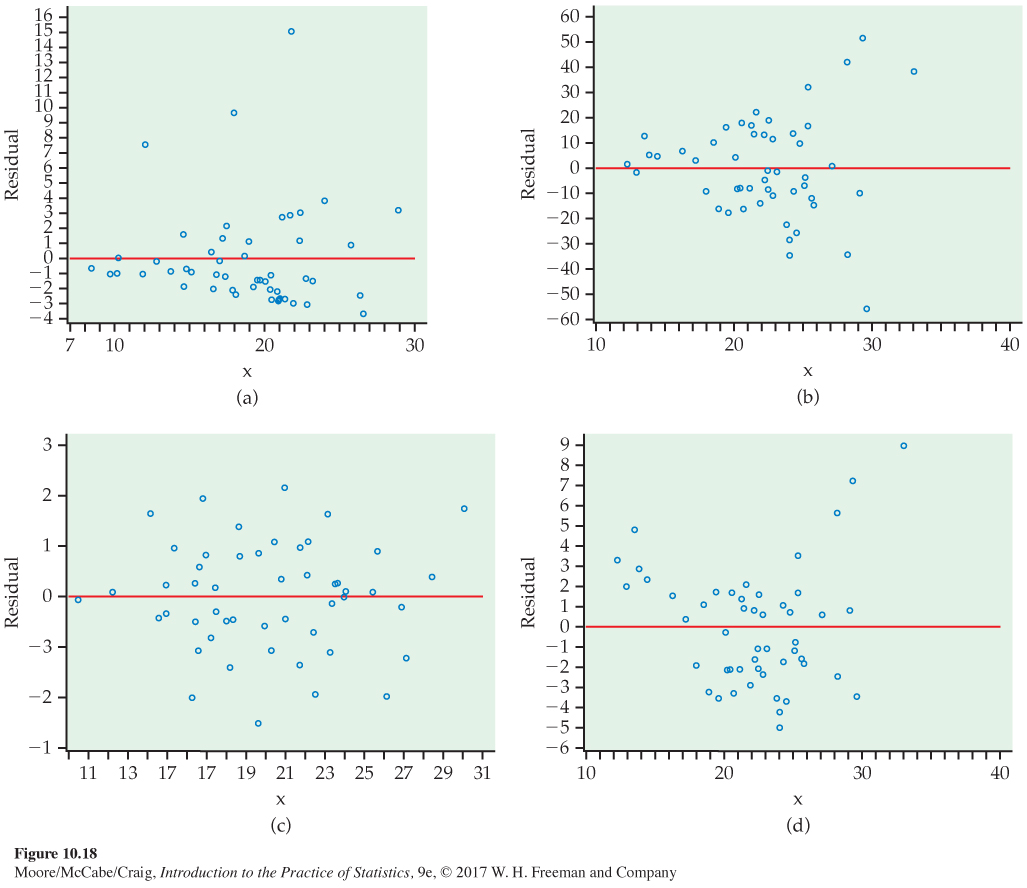 Figure 10.18: FIGURE 10.18 Four plots of residuals versus x, Exercise 10.35.
(b) The following table summarizes the pairwise correlations among the four variables. For each pair of variables, test the null hypothesis that the correlation is zero. Make sure to state the test statistic, degrees of freedom, and P-value.
GPA Anxiety GLS CPU −0.203 0.096 0.012 GPA 0.004 0.207 Anxiety −0.221 (c) Write a short paragraph that summarizes your findings.
Question 10.37
10.37 Beer and blood alcohol. How well does the number of beers a student drinks predict his or her blood alcohol content (BAC)? Sixteen student volunteers at Ohio State University drank a randomly assigned number of 12-
| Student | 1 | 2 | 3 | 4 | 5 | 6 | 7 | 8 |
| Beers | 5 | 2 | 9 | 8 | 3 | 7 | 3 | 5 |
| BAC | 0.10 | 0.03 | 0.19 | 0.12 | 0.04 | 0.095 | 0.07 | 0.06 |
| Student | 9 | 10 | 11 | 12 | 13 | 14 | 15 | 16 |
| Beers | 3 | 5 | 4 | 6 | 5 | 7 | 1 | 4 |
| BAC | 0.02 | 0.05 | 0.07 | 0.10 | 0.085 | 0.09 | 0.01 | 0.05 |
The students were equally divided between men and women and differed in weight and usual drinking habits. Because of this variation, many students don’t believe that number of drinks predicts BAC well.
(a) Make a scatterplot of the data. Find the equation of the least-
squares regression line for predicting BAC from number of beers and add this line to your plot. What is r2 for these data? Briefly summarize what your data analysis shows.(b) Is there significant evidence that drinking more beers increases BAC on the average in the population of all students? State hypotheses, give a test statistic and P-value, and state your conclusion.
(c) Steve thinks his BAC will be below the legal limit to drive 30 minutes after he drinks five beers. The legal limit is BAC = 0.08. Give a 90% prediction interval for Steve’s BAC. Can he be confident he won’t be above the legal limit?
10.37 (a) ˆy = − 0.01270 + 0.01796x; r2 = 79.98%. (b) H0: β1 = 0, Hα: β1 ≠ 0; t = 7.48, P-value < 0.0001. (c) (0.04, 0.1142). He can’t be confident he won’t be arrested.
Question 10.38
10.38 Public university tuition: 2008 versus 2014. Table 10.2 shows the in-
(a) Plot the data with the 2008 tuition on the x axis and describe the relationship. Are there any outliers or unusual values? Does a linear relationship between the tuition in 2008 and 2014 seem reasonable?
(b) Run the simple linear regression and give the least-
squares regression line. (c) Obtain the residuals and plot them versus the 2008 tuition amount. Is there anything unusual in the plot?
(d) Do the residuals appear to be approximately Normal? Explain.
(e) The five California schools appear to follow the same linear trend as the other schools but have higher-
than- predicted in- state tuition in 2014. Assume that this jump is particular to this state (financial troubles?) and remove these five cases and refit the model. How do the parameter estimates change? (f) If you were to move forward with inference, which of these two model fits would you use? Write a short paragraph explaining your answer.
Question 10.39
10.39 More on public university tuition. Refer to the previous exercise. We’ll now move forward with inference using the model fit you chose in part (f) of the previous exercise.
(a) Give the null and alternative hypotheses for examining if there is a linear relationship between 2008 and 2014 tuition amounts.
(b) Write down the test statistic and P-value for the hypotheses stated in part (a). State your conclusions.
(c) Construct a 95% confidence interval for the slope. What does this interval tell you about the annual percent increase in tuition between 2008 and 2014?
(d) What percent of the variability in 2014 tuition is explained by a linear regression model using the 2008 tuition?
(e) Explain why inference on β0 is not of interest for this problem.
10.39 (a) H0: β1 = 0, Hα : β1 ≠ 0. (b) t = 10.67, P-value < 0.0001. (c) (0.83963, 1.24033). (d) r2 = 81.41%. (e) The intercept represents the tuition at x = 0; this is extrapolation.
Question 10.40
10.40 Even more on public university tuition. Refer to the previous two exercises.
(a) The tuition at Skinflint U was $8800 in 2008. What is the predicted tuition in 2014?
Table : TABLE 10.2 In-state Tuition and Fees (in Dollars) for 33 Public Universities School 2008 2014 School 2008 2014 School 2008 2014 Penn State 137067 17955 Ohio State 8679 10995 Texas 8532 11094 Pittsburgh 13642 18075 Virginia 9300 13373 Nebraska 6584 8724 Michigan 11037 14126 Cal- Davis 8635 15589 Iowa 6544 8807 Rutgers 11540 14297 Cal- Berkeley 7656 14421 Colorado 7278 10388 Michigan State 10214 13771 Cal- Irvine 8046 14686 Iowa State 6360 8430 Maryland 8005 9734 Purdue 7750 10868 North Carolina 5397 8616 Illinois 12106 15938 Cal- San Diego 8062 14785 Kansas 7042 10760 Minnesota 10756 14889 Oregon 6435 10254 Arizona 5542 11205 Missouri 8467 10186 Wisconsin 7564 11429 Florida 3778 6748 Buffalo 6285 8784 Washington 6802 13757 Georgia Tech 6040 11094 Indiana 8231 10991 UCLA 7551 14224 Texas A&M 7844 9461 (b) The tuition at I.O.U. was $15,700 in 2008. What is the predicted tuition in 2014?
(c) Discuss the appropriateness of using the fitted equation to predict tuition for each of these universities.
Question 10.41
10.41 Predicting public university tuition: 2000 versus 2014. Refer to Exercise 10.39. The data file also includes the in-
(a) Run the simple linear regression using year 2000 in place of year 2008. What is the least-
squares line? (b) Obtain the residuals and check model assumptions.
(c) If you had to choose between the model using 2008 tuition and the model using 2000 tuition, which would you choose? Give reasons for your answers.
10.41 (a) ˆy = 4466.19453 + 1.70030x. (b) The residual plot looks good; the assumptions are valid.
Question 10.42
10.42 U.S. versus overseas stock returns. Returns on common stocks in the United States and overseas appear to be growing more closely correlated as economies become more interdependent. Suppose that the following population regression line connects the total annual returns (in percent) on two indexes of stock prices:
MEAN OVERSEAS RETURN = −0.08 + 0.20 × U.S.RETURN
(a) What is β0 in this line? What does this number say about overseas returns when the U.S. market is flat (0% return)?
(b) What is β1 in this line? What does this number say about the relationship between U.S. and overseas returns?
(c) We know that overseas returns will vary in years when U.S. returns do not vary. Write the regression model based on the population regression line given above. What part of this model allows overseas returns to vary when U.S. returns remain the same?
Question 10.43
10.43 Performance bonuses. In the National Football League (NFL), performance bonuses now account for roughly 25% of player compensation.18 Does tying a player’s salary into performance bonuses result in better individual or team success on the field? Focusing on linebackers, let’s look at the relationship between a player’s end-
(a) Use numerical and graphical methods to describe the two variables and summarize your results.
(b) Both variable distributions are non-
Normal. Does this necessarily pose a problem for performing linear regression? Explain. (c) Construct a scatterplot of the data and describe the relationship. Are there any outliers or unusual values? Does a linear relationship between the percent of salary and the player rating seem reasonable? Is it a very strong relationship? Explain.
(d) Run the simple linear regression and state the least-
squares regression line. (e) Obtain the residuals and assess whether the assumptions for the linear regression analysis are reasonable. Include all plots and numerical summaries used in doing this assessment.
10.43 (a) Both distributions are also right-skewed; the five-number summaries are 0%, 0.31%, 1.43%, 17.65%, 85.01% and 0, 2.25, 6.31, 12.69, 27.88. (b) Only the residuals need to be Normal. (c) The relationship is quite scattered. (d) ˆy = 6.24693 + 0.10634x. (e) The residuals are right-skewed.
Question 10.44
![]() 10.44 Performance bonuses, continued. Refer to the previous exercise.
10.44 Performance bonuses, continued. Refer to the previous exercise.
(a) Now run the simple linear regression for the variables sqrt(rating) and percent of salary devoted to incentive payments.
(b) Obtain the residuals and assess whether the assumptions for the linear regression analysis are reasonable. Include all plots and numerical summaries used in doing this assessment.
(c) Construct a 95% confidence interval for the square root increase in rating given a 1% increase in the percent of salary devoted to incentive payments.
(d) Consider the values 0%, 20%, 40%, 60%, and 80% salary devoted to incentives. Compute the predicted rating for this model and for the one in the previous exercise. For the model in this problem, you will need to square the predicted value to get back to the original units.
(e) Plot the predicted values versus the percent and connect those values from the same model. For which regions of percent do the predicted values from the two models differ the most?
(f) Based on the comparison of regression models (both predicted values and residuals), which model do you prefer? Explain.
Question 10.45
10.45 Sales price versus assessed value. Real estate is typically reassessed annually for property tax purposes. This assessed value, however, is not necessarily the same as the fair market value of the property. Table 10.3 summarizes an SRS of 35 homes recently sold in a midwestern city.19 Both variables are measured in thousands of dollars.
(a) Inspect the data. How many homes have a sales price greater than the assessed value? Do you think this trend would be true for the larger population of all homes recently sold? Explain your answer.
(b) Make a scatterplot with assessed value on the horizontal axis. Briefly describe the relationship between assessed value and sales price.
(c) Based on the scatterplot, there is one distinctly unusual observation. State which property it is, and describe the impact you expect this observation has on the least-
squares line. Table : TABLE 10.3 Sales Price and Assessed Value (in Thousands of $) of 35 Homes in a Midwestern CityProperty Sales
priceAssessed
valueProperty Sales
priceAssessed
valueProperty Sales
priceAssessed
value1 83.0 87.0 13 249.9 192.0 25 146.0 121.1 2 129.9 103.8 14 112.0 117.4 26 230.5 212.1 3 125.0 111.0 15 133.0 117.2 27 360.0 167.9 4 245.0 157.4 16 177.5 116.6 28 127.9 110.2 5 100.0 127.5 17 162.5 143.7 29 205.0 183.2 6 134.7 127.7 18 238.0 198.2 30 163.5 93.6 7 106.0 110.9 19 120.9 93.4 31 225.0 156.2 8 91.5 90.8 20 142.5 92.3 32 335.0 278.1 9 170.0 160.7 21 299.0 279.0 33 192.0 151.0 10 295.0 250.5 22 82.5 90.4 34 232.0 178.8 11 179.0 160.9 23 152.5 103.2 35 197.9 172.4 12 230.0 213.2 24 139.9 114.9 (d) Report the least-
squares regression line for predicting selling price from assessed value using all 35 properties. What is the estimated model standard error? (e) Now remove the unusual observation and fit the data again. Report the least-
squares regression line and estimated model standard error. (f) Compare the two sets of results. Describe the impact this unusual observation has on the results.
(g) Do you think it is more appropriate to consider all 35 properties for linear regression analysis or just consider the 34 properties? Explain your decision.
10.45 (a) 30. (b) The relationship is linear, positive, and strong. (c) House 27 is unusual and could be influential. (d) ˆy = 9.0176 + 1.15705x, s = 37.34442. (e) ˆy = 9.43181 + 1.123x, s = 25.39177. (f) The outlier has some influence; the first model has a much larger standard error.
Question 10.46
10.46 Sales price versus assessed value, continued. Refer to the previous exercise. Let’s consider linear regression analysis using just 34 properties.
(a) Obtain the residuals and plot them versus assessed value. Is there anything unusual to report? If so, explain.
(b) Do the residuals appear to be approximately Normal? Describe how you assessed this.
(c) Based on your answers to parts (a) and (b), do you think the assumptions for statistical inference are reasonably satisfied? Explain your answer.
(d) Construct a 95% confidence interval for the slope and summarize the results.
(e) Using the result from part (d), compare the estimated regression line with y = x, which says that, on average, the selling price is equal to the assessed value. Is there evidence that this model is not reasonable? In other words, is the selling price typically larger or smaller than the assessed value? Explain your answer.
Question 10.47
10.47 Gambling and alcohol use by first-
(a) What percent of the variability in AUDIT score is explained by frequency of gambling?
(b) Test the null hypothesis that the correlation between the gambling frequency and the AUDIT score is zero.
(c) The sample in this study represents 45% of the students contacted for the online study. To what extent do you think these results apply to all first-
year students at this university? To what extent do you think these results apply to all first- year students? Give reasons for your answers.
10.47 (a) 8.41%. (b) H0: ρ = 0. Hα: ρ ≠ 0. t = 9.12, P-value < 0.0001. (c) Students who did not answer might have different characteristics.
Question 10.48
![]() 10.48 Predicting water quality. The index of biotic integrity (IBI) is a measure of the water quality in streams. IBI and land use measures for a collection of streams in the Ozark Highland ecoregion of Arkansas were collected as part of a study.21 Table 10.4 gives the data for IBI, the percent of the watershed that was forest, and the area of the watershed in square kilometers for streams in the original sample with watershed area less than or equal to 70 km2.
10.48 Predicting water quality. The index of biotic integrity (IBI) is a measure of the water quality in streams. IBI and land use measures for a collection of streams in the Ozark Highland ecoregion of Arkansas were collected as part of a study.21 Table 10.4 gives the data for IBI, the percent of the watershed that was forest, and the area of the watershed in square kilometers for streams in the original sample with watershed area less than or equal to 70 km2.
(a) Use numerical and graphical methods to describe the variable IBI. Do the same for area. Summarize your results.
Table : TABLE 10.4 Watershed Area (km2), Percent Forest, and Index of Biotic IntegrityArea Forest IBI Area Forest IBI Area Forest IBI Area Forest IBI Area Forest IBI 21 0 47 29 0 61 31 0 39 32 0 59 34 0 72 34 0 76 49 3 85 52 3 89 2 7 74 70 8 89 6 9 33 28 10 46 21 10 32 59 11 80 69 14 80 47 17 78 8 17 53 8 18 43 58 21 88 54 22 84 10 25 62 57 31 55 18 32 29 19 33 29 39 33 54 49 33 78 9 39 71 5 41 55 14 43 58 9 43 71 23 47 33 31 49 59 18 49 81 16 52 71 21 52 75 32 59 64 10 63 41 26 68 82 9 75 60 54 79 84 12 79 83 21 80 82 27 86 82 23 89 86 26 90 79 16 95 67 26 95 56 26 100 85 28 100 91 (b) Plot the data and describe the relationship between IBI and area. Are there any outliers or unusual patterns?
(c) Give the statistical model for simple linear regression for this problem.
(d) State the null and alternative hypotheses for examining the relationship between IBI and area.
(e) Run the simple linear regression and summarize the results.
(f) Obtain the residuals and plot them versus area. Is there anything unusual in the plot?
(g) Do the residuals appear to be approximately Normal? Give reasons for your answer.
(h) Do the assumptions for the analysis of these data using the model you gave in part (c) appear to be reasonable? Explain your answer.
Question 10.49
![]() 10.49 More on predicting water quality. The researchers who conducted the study described in the previous exercise also recorded the percent of the watershed area that was forest for each of the streams. These data are also given in Table 10.4. Analyze these data using the questions in the previous exercise as a guide.
10.49 More on predicting water quality. The researchers who conducted the study described in the previous exercise also recorded the percent of the watershed area that was forest for each of the streams. These data are also given in Table 10.4. Analyze these data using the questions in the previous exercise as a guide.
10.49 (a) IBI is slightly left-skewed; ˉx = 65.94, s = 18.28; Forest is slightly right-skewed; ˉx = 28.29, s = 17.71.
(b) A weak positive association.
(c) yi=β0+β1xi+∈i, ∈i~N(0, σ).
(d) H0:β1=0, Hα:β1≠0.
(e) ˆy = 59.91 + 0.1531Forest, s = 17.79. t = 1.92, P-value = 0.0608.
(f) The residual plot shows that there is more variation for small x.
(g) The residuals seem reasonably close to Normal.
Question 10.50
10.50 Comparing the analyses. In Exercises 10.48 and 10.49, you used two different explanatory variables to predict IBI. Summarize the two analyses and compare the results. If you had to choose between the two explanatory variables for predicting IBI, which one would you prefer? Give reasons for your answer.
Question 10.51
10.51 How an outlier can affect statistical significance. Consider the data in Table 10.4 and the relationship between IBI and the percent of watershed area that was forest. The relationship between these two variables is almost significant at the 0.05 level. In this exercise, you will demonstrate the potential effect of an outlier on statistical significance. Investigate what happens when you decrease the IBI to 0.0 for (1) an observation with 0% forest and (2) an observation with 100% forest. Write a short summary of what you learn from this exercise.
10.51 The first change decreases P (that is, the relationship is more significant) because it accentuates the positive association. The second change weakens the association, so P increases (the relationship is less significant).
Question 10.52
10.52 Predicting water quality for an area of 40 km2. Refer to Exercise 10.48.
(a) Find a 95% confidence interval for the mean response corresponding to an area of 40 km2.
(b) Find a 95% prediction interval for a future response corresponding to an area of 40 km2.
(c) Write a short paragraph interpreting the meaning of the intervals in terms of Ozark Highland streams.
(d) Do you think that these results can be applied to other streams in Arkansas or in other states? Explain why or why not.
Question 10.53
10.53 Compare the predictions. Refer to Exercise 10.50. Another way to compare analyses is to compare predictions. Consider Case 37 in Table 10.4 (8th row, 2nd column). For this case, the area is 10 km2 and the percent forest is 63%. Calculate the predicted index of biotic integrity based on area and the predicted index of biotic integrity based on percent forest. Compare these two predictions and explain why they differ. Use the idea of a prediction interval to interpret these results.
10.53 Using area: 57.52; (23.5598, 91.4892). Using forest: 69.55; (33.2085, 105.9006). Both prediction intervals have a lot of error.
Question 10.54
10.54 Reading test scores and IQ. For a study of reading ability in schoolchildren, researchers collected reading test scores and IQ scores for a sample of 60 fifth-
(a) Run the regression and summarize the results of the significance tests.
(b) Rerun the analysis with the four possible outliers removed. Summarize your findings, paying particular attention to the effects of removing the outliers.
Question 10.55
10.55 Leaning Tower of Pisa. The Leaning Tower of Pisa is an architectural wonder. Engineers concerned about the tower’s stability have done extensive studies of its increasing tilt. Measurements of the lean of the tower over time provide much useful information. The following table gives measurements for the years 1975 to 1987. The variable “lean’’ represents the difference between where a point on the tower would be if the tower were straight and where it actually is. The data are coded as tenths of a millimeter in excess of 2.9 meters, so that the 1975 lean, which was 2.9642 meters, appears in the table as 642. Only the last two digits of the year were entered into the computer.23
| Year | 75 | 76 | 77 | 78 | 79 | 80 | 81 | 82 | 83 | 84 | 85 | 86 | 87 |
| Lean | 642 | 644 | 656 | 667 | 673 | 688 | 696 | 698 | 713 | 717 | 725 | 742 | 757 |
(a) Plot the data. Does the trend in lean over time appear to be linear?
(b) What is the equation of the least-
squares line? What percent of the variation in lean is explained by this line? (c) Give a 99% confidence interval for the average rate of change (tenths of a millimeter per year) of the lean.
10.55 (a) Very linear. (b) ˆy = − 61.12 + 9.3187Year; r2 = 98.8%. (c) (8.3562, 10.2812).
Question 10.56
10.56 More on the Leaning Tower of Pisa. Refer to the previous exercise.
(a) In 1918 the lean was 2.9071 meters. (The coded value is 71.) Using the least-
squares equation for the years 1975 to 1987, calculate a predicted value for the lean in 1918. (Note that you must use the coded value 18 for year.) (b) Although the least-
squares line gives an excellent fit to the data for 1975 to 1987, this pattern did not extend back to 1918. Write a short statement explaining why this conclusion follows from the information available. Use numerical and graphical summaries to support your explanation.
Question 10.57
10.57 Predicting the lean in 2016. Refer to the previous two exercises.
(a) How would you code the explanatory variable for the year 2016?
(b) The engineers working on the Leaning Tower of Pisa were most interested in how much the tower would lean if no corrective action was taken. Use the least-
squares equation to predict the tower’s lean in the year 2016. (Note: The tower was renovated in 2001 to make sure it does not fall down.) (c) To give a margin of error for the lean in 2016, would you use a confidence interval for a mean response or a prediction interval? Explain your choice.
10.57 (a) 116. (b) ˆy = 1019.8492, for a prediction of 3.0020 m. (c) Prediction interval.
Question 10.58
10.58 Does a math pretest predict success? Can a pretest on mathematics skills predict success in a statistics course? The 62 students in an introductory statistics class took a pretest at the beginning of the semester. The least-
(a) Test the null hypothesis that there is no linear relationship between the pretest score and the score on the final exam against the two-
sided alternative .(b) Would you reject this null hypothesis versus the one-
sided alternative that the slope is positive? Explain your answer.
Question 10.59
10.59 Significance test of the correlation. A study reported a correlation r = 0.5 based on a sample size of n = 15; another reported the same correlation based on a sample size of n = 25. For each, perform the test of the null hypothesis that ρ = 0. Describe the results and explain why the conclusions are different.
10.59 For n = 15, t = 2.08; for n = 25, t = 2.77. The P-values are 0.0579 and 0.0109. Finding the same correlation with more data points is stronger evidence that the observed correlation is not just due to chance.
Question 10.60
10.60 State and college binge drinking. Excessive consumption of alcohol is associated with numerous adverse consequences. In one study, researchers analyzed binge-
(a) Find the equation of the least-
squares line for predicting the college binge- drinking rate from the adult binge- drinking rate. (b) Give the results of the significance test for the null hypothesis that the slope is 0. ( Hint: What is the relation between this test and the test for a zero correlation?)
Question 10.61
10.61 SAT versus ACT. The SAT and the ACT are the two major standardized tests that colleges use to evaluate candidates. Most students take just one of these tests. However, some students take both. Consider the scores of 60 students who did this. How can we relate the two tests?
(a) Plot the data with SAT on the x axis and ACT on the y axis. Describe the overall pattern and any unusual observations.
(b) Find the least-
squares regression line and draw it on your plot. Give the results of the significance test for the slope. (c) What is the correlation between the two tests?
10.61 (a) Strong, positive linear relationship with one outlier. (b) ˆy = 1.63 + 0.0214SAT. t = 10.78, P-value < 0.0005. (c) r = 0.8167.
Question 10.62
![]() 10.62 SAT versus ACT, continued. Refer to the previous exercise. Find the predicted value of ACT for each observation in the data set.
10.62 SAT versus ACT, continued. Refer to the previous exercise. Find the predicted value of ACT for each observation in the data set.
(a) What is the mean of these predicted values? Compare it with the mean of the ACT scores.
(b) Compare the standard deviation of the predicted values with the standard deviation of the actual ACT scores. If least-
squares regression is used to predict ACT scores for a large number of students such as these, the average predicted value will be accurate, but the variability of the predicted scores will be too small. (c) Find the SAT score for a student who is 1 standard deviation above the mean (z=(x−ˉx)/sx=1). Find the predicted ACT score and standardize this score. (Use the means and standard deviations from this set of data for these calculations.)
(d) Repeat part (c) for a student whose SAT score is 1 standard deviation below the mean (z = −1).
(e) What do you conclude from parts (c) and (d)? Perform additional calculations for different z’s if needed.
Question 10.63
![]() 10.63 Matching standardized scores. Refer to the previous two exercises. An alternative to the least-
10.63 Matching standardized scores. Refer to the previous two exercises. An alternative to the least-
(y−ˉy)sy=(x−ˉx)sx
and solve for y. Let’s use the notation y = a0 + a1x for this line. The slope is a1=sy/sx and the intercept is a0=ˉy−a1ˉx. Compare these expressions with the formulas for the least-
(a) Using the data in the previous exercise, find the values of a0 and a1.
(b) Plot the data with the least-
squares line and the new prediction line. (c) Use the new line to find predicted ACT scores. Find the mean and the standard deviation of these scores. How do they compare with the mean and standard deviation of the ACT scores?
10.63 (a) α1 = 0.02617, α0 = − 2.7522. (c) ˉy = 21.13 and sy = 4.7137.
Question 10.64
![]() 10.64 Index of biotic integrity. Refer to the data on the index of biotic integrity and area in Exercise 10.48 (page 602) and the additional data on percent watershed area that was forest in Exercise 10.49. Find the correlations among these three variables, perform the test of statistical significance, and summarize the results. Which of these test results could have been obtained from the analyses that you performed in Exercises 10.48 and 10.49?
10.64 Index of biotic integrity. Refer to the data on the index of biotic integrity and area in Exercise 10.48 (page 602) and the additional data on percent watershed area that was forest in Exercise 10.49. Find the correlations among these three variables, perform the test of statistical significance, and summarize the results. Which of these test results could have been obtained from the analyses that you performed in Exercises 10.48 and 10.49?
Question 10.65
10.65 A mechanistic explanation of popularity. Previous experimental work has suggested that the serotonin system plays an important and causal role in social status. In other words, genes may predispose individuals to be popular/likable. As part of a recent study on adolescents, an experimenter looked at the relationship between the expression of a particular serotonin receptor gene, a person’s “popularity,’’ and the person’s rule-
| Rule- |
Popularity | Gene expression |
| Sample 1 (n = 123) | ||
| RB.composite | 0.28 | 0.26 |
| RB.questionnaire | 0.22 | 0.23 |
| RB.video | 0.24 | 0.20 |
| Sample 1 Caucasians only (n = 96) | ||
| RB.composite | 0.22 | 0.23 |
| RB.questionnaire | 0.16 | 0.24 |
| RB.video | 0.19 | 0.16 |
For each correlation, test the null hypothesis that the corresponding true correlation is zero. Reproduce the table and mark the correlations that have P < 0.001 with ***, those that have P < 0.01 with **, and those that have P < 0.05 with *. Write a summary of the results of your significance tests.
10.65 For n = 123: between 0.24 and 0.28 have a P-value < 0.01; between 0.20 and 0.23 have a P-value < 0.05. For n = 96: between 0.22 and 0.24 have a P-value < 0.05; the others are not significant.
Question 10.66
10.66 Resting metabolic rate and exercise. Metabolic rate, the rate at which the body consumes energy, is important in studies of weight gain, dieting, and exercise. The following table gives data on the lean body mass and resting metabolic rate for 12 women and seven men who are subjects in a study of dieting. Lean body mass, given in kilograms, is a person’s weight leaving out all fat. Metabolic rate is measured in calories burned per 24 hours, the same calories used to describe the energy content of foods. The researchers believe that lean body mass is an important influence on metabolic rate.
| Subject | Sex | Mass | Rate | Subject | Sex | Mass | Rate |
| 1 | M | 62.0 | 1792 | 11 | F | 40.3 | 1189 |
| 2 | M | 62.9 | 1666 | 12 | F | 33.1 | 913 |
| 3 | F | 36.1 | 995 | 13 | M | 51.9 | 1460 |
| 4 | F | 54.6 | 1425 | 14 | F | 42.4 | 1124 |
| 5 | F | 48.5 | 1396 | 15 | F | 34.5 | 1052 |
| 6 | F | 42.0 | 1418 | 16 | F | 51.1 | 1347 |
| 7 | M | 47.4 | 1362 | 17 | F | 41.2 | 1204 |
| 8 | F | 50.6 | 1502 | 18 | M | 51.9 | 1867 |
| 9 | F | 42.0 | 1256 | 19 | M | 46.9 | 1439 |
| 10 | M | 48.7 | 1614 |
(a) Make a scatterplot of the data, using different symbols or colors for men and women. Summarize what you see in the plot.
(b) Run the regression to predict metabolic rate from lean body mass for the women in the sample and summarize the results. Do the same for the men.
Question 10.67
![]() 10.67 Resting metabolic rate and exercise, continued. Refer to the previous exercise. It is tempting to conclude that there is a strong linear relationship for the women but no relationship for the men. Let’s look at this issue a little more carefully.
10.67 Resting metabolic rate and exercise, continued. Refer to the previous exercise. It is tempting to conclude that there is a strong linear relationship for the women but no relationship for the men. Let’s look at this issue a little more carefully.
(a) Find the confidence interval for the slope in the regression equation that you ran for the females. Do the same for the males. What do these suggest about the possibility that these two slopes are the same? (The formal method for making this comparison is a bit complicated and is beyond the scope of this chapter.)
(b) Examine the formula for the standard error of the regression slope given on page 591. The term in the denominator is √∑(xi−ˉx)2. Find this quantity for the females; do the same for the males. How do these calculations help to explain the results of the significance tests?
(c) Suppose that you were able to collect additional data for males. How would you use lean body mass in deciding which subjects to choose?
10.67 (a) For women: (14.72609, 33.32604). For men: ( − 9.46079, 42.96351). These intervals overlap quite a bit. (b) For women: 22.78. For men: 16.38.The women’s standard error is smaller in part because it is divided by a larger n. (c) Choose men with a wider variety of lean body masses.