608

Population multiple regression equation

The simple linear regression model assumes that the mean of the response variable y depends on the explanatory variable x according to a linear equation

μ_y = β₀ + β₁x

For any fixed value of x, the response y varies Normally about this mean and has a standard deviation σ that is the same for all values of x.

In the multiple regression setting, the response variable y depends on p explanatory variables, which we will denote by x₁, x₂, … , x_p. The mean response depends on these explanatory variables according to a linear function

μ_y = β₀ + β₁x₁ + β₂x₂ + … + β_px_p

Similar to simple linear regression, this expression is the population regression equationpopulation regression equation, and the observed values y vary about their means given by this equation.

Just as we did in simple linear regression, we can also think of this model in terms of subpopulations of responses. Here, each subpopulation corresponds to a particular set of values for all the explanatory variables x₁, x₂, … , x_p. In each subpopulation, y varies Normally with a mean given by the population regression equation. The regression model assumes that the standard deviation σ of the responses is the same in all subpopulations.

Data for multiple regression

The data for a simple linear regression problem consist of observations (x_i, y_i) of the two variables. Because there are several explanatory variables in multiple regression, the notation needed to describe the data is more elaborate. Each observation or case consists of a value for the response variable and for each of the explanatory variables. Call the value of the jth explanatory variable for the ith case. The data are then

Here, n is the number of cases and p is the number of explanatory variables. Data are often entered into computer regression programs in this format. Each row is a case and each column corresponds to a different variable.

The data for Example 11.1, with several additional explanatory variables, appear in this format in the GPA data file. Figure 11.1 shows the first six rows entered into an Excel spreadsheet. Grade point average (GPA) is the response variable, followed by p = 7 explanatory variables, six achievement scores and sex. There are a total of n = 150 students in this data set.

610

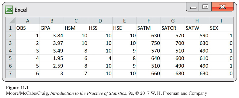
The six achievement scores are all quantitative explanatory variables. SEX is an indicator variableindicator variable using the numeric values 0 and 1 to represent male and female, respectively. Indicator variables are used frequently in multiple regression to represent the levels or groups of a categorical explanatory variable. See Exercise 11.22 (page 635) for more discussion of their use in a multiple regression model.

Multiple linear regression model

Similar to simple linear regression, we combine the population regression equation and the assumptions about how the observed y vary about their means to construct the multiple linear regression model. The subpopulation means describe the FIT part of our conceptual model

DATA = FIT + RESIDUAL

The RESIDUAL part represents the variation of observed y about their means.

We will use the same notation for the residual that we used in the simple linear regression model. The symbol ϵ represents the deviation of an individual observation from its subpopulation mean. We assume that these deviations are Normally distributed with mean 0 and an unknown model standard deviation σ that does not depend on the values of the x variables. These are assumptions that we can check by examining the residuals in the same way that we did for simple linear regression.

The assumption that the subpopulation means are related to the regression coefficients β by the equation

implies that we can estimate all subpopulation means from estimates of the β’s. To the extent that this equation is accurate, we have a useful tool for describing how the mean of y varies with the collection of x’s.

We do, however, need to be cautious when interpreting each of the regression coefficients in a multiple regression. First, the β₀ coefficient represents the mean of y when all the x variables equal zero. Even more so than in simple linear regression, this subpopulation is rarely of interest. Second, the description provided by the regression coefficient of each x variable is similar to that provided by the slope in simple linear regression but only in a specific situation—namely, when all other x variables are held constant. We need this extra condition because with multiple x variables, it is quite possible that a unit change in one x variable may be associated with changes in other x variables. If that occurs, then the overall change in the mean of y is not described by just a single regression coefficient.

Estimation of the multiple regression parameters

Similar to simple linear regression, we use the method of least squares to obtain estimators of the regression coefficients β. Let

b₀, b₁, b₂, … , b_p

denote the estimators of the parameters

β₀, β₁, β₂, … , β_p

For the ith observation, the predicted response is

612

The ith residual, the difference between the observed and the predicted response, is, therefore,

The method of least squares chooses the values of the b’s that make the sum of the squared residuals as small as possible. In other words, the parameter estimates b₀, b₁, b₂, … , b_p minimize the quantity

The formula for the least-squares estimates in multiple regression is complicated. We will be content to understand the principle on which it is based and to let software do the computations.

The parameter σ² measures the variability of the responses about the population regression equation. As in the case of simple linear regression, we estimate σ² by an average of the squared residuals. The estimator is

The quantity n − p − 1 is the degrees of freedom associated with s². The degrees of freedom equal the sample size, n, minus (p + 1), the number of β’s we must estimate to fit the model. In the simple linear regression case, there is just one explanatory variable, so p = 1 and the degrees of freedom are n − 2. To estimate the model standard deviation σ, we use

Confidence intervals and significance tests for regression coefficients

We can obtain confidence intervals and perform significance tests for each of the regression coefficients β_j as we did in simple linear regression. The standard errors of the b’s have more complicated formulas, but all are multiples of the estimated model standard deviation σ. We again rely on statistical software to do the calculations.

Be very careful in your interpretation of the t tests and confidence intervals for individual regression coefficients. In simple linear regression, the model says that μ_y = β₀ + β₁x. The null hypothesis H₀: β₁ = 0 says that regression on x is of no value for predicting the response y or, alternatively, that there is no straight-line relationship between x and y. The corresponding null hypothesis for the multiple regression model μ_y = β₀ + β₁x₁ + β₂x₂ + … + β_px_p says that x₁ is of no value for predicting y, given that x₂, x₃, … , x_p are in the model. In other words, the predictor x₁ contains no additional information over or above that contained in x₂, x₃, … , x_p that is useful for predicting y. This a very important difference and one we will return to when analyzing the data of Example 11.1.

Because regression is often used for prediction, we may wish to use multiple regression models to construct confidence intervals for a mean response and prediction intervals for a future observation. The basic ideas are the same as in the simple linear regression case.

In most software systems, the same commands that give confidence and prediction intervals for simple linear regression work for multiple regression. The only difference is that we specify a list of explanatory variables rather than a single variable. Modern software allows us to perform these rather complex calculations without an intimate knowledge of all the computational details. This frees us to concentrate on the meaning and appropriate use of the results.

ANOVA table for multiple regression

In simple linear regression, the F test from the ANOVA table is equivalent to the two-sided t test of the hypothesis that the slope of the regression line is 0. For multiple regression, there is a corresponding ANOVA F test, but it tests the hypothesis that all the regression coefficients (with the exception of the intercept) are 0. Here is the general form of the ANOVA table for multiple regression:

614

The ANOVA table is similar to that for simple linear regression. The degrees of freedom for the model increase from 1 to p to reflect the fact that we now have p explanatory variables rather than just one. As a consequence, the degrees of freedom for error decrease by the same amount. It is always a good idea to calculate the degrees of freedom by hand and then check that your software agrees with your calculations. This ensures that you have not made some serious error in specifying the model or in entering the data.

The sums of squares represent sources of variation. Once again, both the sums of squares and their degrees of freedom add:

SST = SSM + SSE

DFT = DFM + DFE

The estimate of the variance σ² for our model is again given by the MSE in the ANOVA table. That is, s² = MSE.

The ratio MSM/MSE is an F statistic for testing the null hypothesis

H₀: β₁ = β₂ = … = β_p = 0

against the alternative hypothesis

H_a: at least one of the β_j is not 0

The null hypothesis says that none of the explanatory variables are predictors of the response variable when used in the form expressed by the multiple regression equation. The alternative states that at least one of them is a predictor of the response variable.

As in simple linear regression, large values of F give evidence against H₀. When H₀ is true, F has the F(p, n − p − 1) distribution. The degrees of freedom for the F distribution are those associated with the model and error in the ANOVA table.

A common error in the use of multiple regression is to assume that all the regression coefficients are statistically different from zero whenever the F statistic has a small P-value. Be sure that you understand the difference between the F test and the t tests for individual coefficients in the multiple regression setting.

Squared multiple correlation R²

615

For simple linear regression, we noted that the square of the sample correlation could be written as the ratio of SSM to SST and could be interpreted as the proportion of variation in y explained by x. The ratio of SSM to SST is routinely calculated for multiple regression and still can be interpreted as the proportion of explained variation. The difference is that it relates to the collection of explanatory variables in the model.

Often, R² is multiplied by 100 and expressed as a percent. The square root of R², called the multiple correlation coefficientmultiple correlation coefficient, is the correlation between the observations y_i and the predicted values