11.2 11.2 A Case Study
In this section, we illustrate multiple regression by analyzing the data from the study described in Example 11.1. There are data for n = 150 students. The response variable is the cumulative GPA, on a four-
Before starting the analysis, we first consider the extent to which our results can be generalized. For this study, all the available data are being analyzed. There is no random sampling from the population of science majors. In this setting, we often justify the use of inference by viewing the data as coming from some sort of process. Here, we consider this collection of students as a sample of all the science majors who will attend this university. Still, opinions may vary as to the extent to which these data can be considered an SRS sample of current and future students. For example, schools seem to consistently brag that their new batch of first-
Preliminary analysis
As with any statistical analysis, we begin our multiple regression with a careful examination of the data. We first look at each variable separately, then at relationships among the variables. In both cases, we continue our practice of combining plots and numerical descriptions. We use JMP, Excel, SAS, Minitab, and SPSS to illustrate the outputs that are given by most software.
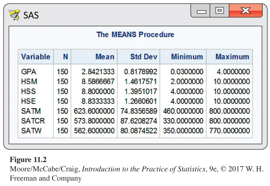
Means, standard deviations, and minimum and maximum values appear in Figure 11.2. The minimum value for high school mathematics (HSM) appears to be rather extreme; it is |2.00 − 8.59|/1.46 = 4.51 standard deviations below the mean. Similarly, the minimum value for GPA is 3.43 standard deviations below the mean. We do not discard either of these cases at this time but will take care in our subsequent analyses to see if they have an excessive influence on our results.
The mean for the SATM score is higher than the means for the Critical Reading (SATCR) and Writing (SATW) scores, as we might expect for a group of science majors. The three SAT standard deviations are all about the same.
Although mathematics scores were higher on the SAT, the means and standard deviations of the three high school grade variables are very similar. Because the level and difficulty of high school courses vary within and across schools, this may not be that surprising. The mean GPA is 2.842 on a four-
![]()
Because the variables GPA, SATM, SATCR, and SATW have many possible values, we could use stemplots or histograms to examine the shapes of their distributions. Normal quantile plots indicate whether or not the distributions look Normal. It is important to note that the multiple regression model does not require any of these distributions to be Normal. Only the deviations of the responses y from their means are assumed to be Normal.
![]()
The purpose of examining these plots is to understand something about each variable alone before attempting to use it in a complicated model. Extreme values of any variable should be noted and checked for accuracy. If found to be correct, the cases with these values should be carefully examined to see if they are truly exceptional and perhaps do not belong in the same analysis with the other cases. When our data on science majors are examined in this way, no obvious problems are evident.
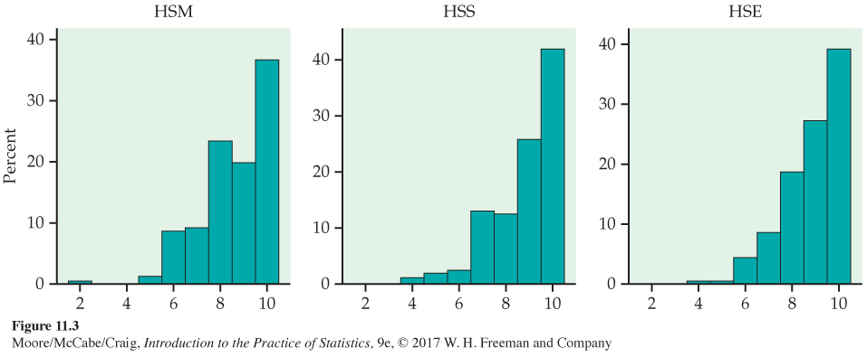
The high school grade variables HSM, HSS, and HSE take only integer values. The bar plots using relative frequencies are shown in Figure 11.3. The distributions are all skewed, with a large proportion of high grades (10 = A and 9 = A−). Again we emphasize that these distributions need not be Normal.
correlation, p. 101
Relationships between pairs of variables
The second step in our analysis is to examine the relationships between all pairs of variables. Scatterplots and correlations are our tools for studying two-
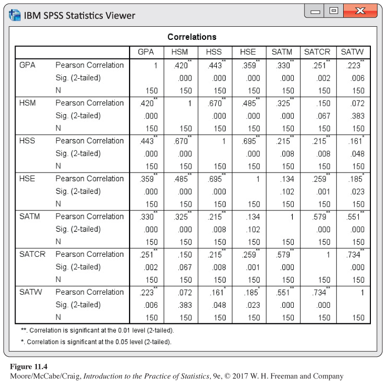
As we might expect, math and science grades have the highest correlation with GPA (r = 0.420 and r = 0.443), followed by English grades (0.359) and then SAT Mathematics (0.330). SAT Critical Reading (SATCR) and SAT Writing (SATW) have comparable, somewhat weak, correlations with GPA. On the other hand, SATCR and SATW have a high correlation with each other (0.734). The high school grades also correlate well with each other (0.485 to 0.695). SATM correlates well with the other SAT scores (0.579 and 0.551), somewhat with HSM (0.325), less with HSS (0.215), and poorly with HSE (0.134). SATCR and SATW do not correlate well with any of the high school grades (0.072 to 0.259).
![]()
It is important to keep in mind that, by examining pairs of variables, we are seeking a better understanding of the data. The fact that the correlation of a particular explanatory variable with the response variable does not achieve statistical significance does not necessarily imply that it will not be a useful (and statistically significant) predictor in a multiple regression model.
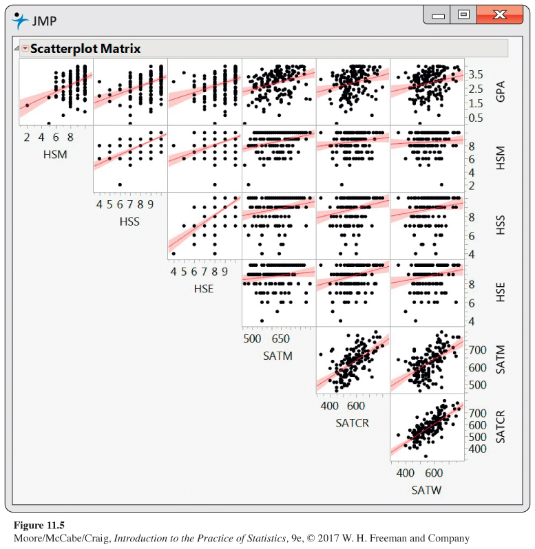
Numerical summaries such as correlations are useful, but plots are generally more informative when seeking to understand data. Plots tell us whether the numerical summary gives a fair representation of the data.
![]()
For a multiple regression, each pair of variables should be plotted. For the seven variables in our case study, this means that we should examine 21 plots. In general, there are p + 1 variables in a multiple regression analysis with p explanatory variables, so that p(p + 1)/2 plots are required. Multiple regression is a complicated procedure. If we do not do the necessary preliminary work, we are in serious danger of producing useless or misleading results.
USE YOUR KNOWLEDGE
Question 11.13
11.13 Pairwise relationships among variables in the GPA data set. Most statistical software packages have the option to create a “scatterplot matrix’’ of all p(p + 1)/2 scatterplots. For example, in JMP, there is the option “Scatterplot Matrix’’ under the Graph menu. Figure 11.5 is the scatterplot matrix for the GPA data, including the least-
11.13 Answers will vary. Scatterplots are visual, the correlation matrix gives the actual values.
Regression on high school grades
To explore the relationship between the explanatory variables and our response variable GPA, we run several multiple regressions. The explanatory variables fall into three classes. High school grades are represented by HSM, HSS, and HSE; standardized tests are represented by the three SAT scores; and sex of the student is represented by SEX. We begin our analysis by using the high school grades to predict GPA. Figure 11.6 gives the multiple regression output.
The output contains an ANOVA table, some additional fit statistics, and information about the parameter estimates. Because there are n = 150 cases, we have DFT = n − 1 = 149. The three explanatory variables give DFM = p = 3 and DFE = n − p − 1 = 150 − 3 − 1 = 146.
The ANOVA F statistic is 14.35, with a P-value of <0.0001. Under the null hypothesis
H0: β1 = β2 = β3 = 0
the F statistic has an F(3, 146) distribution. According to this distribution, the chance of obtaining an F statistic of 14.35 or larger is less than 0.0001. Therefore, we conclude that at least one of the three regression coefficients for the high school grades is different from 0 in the population regression equation.
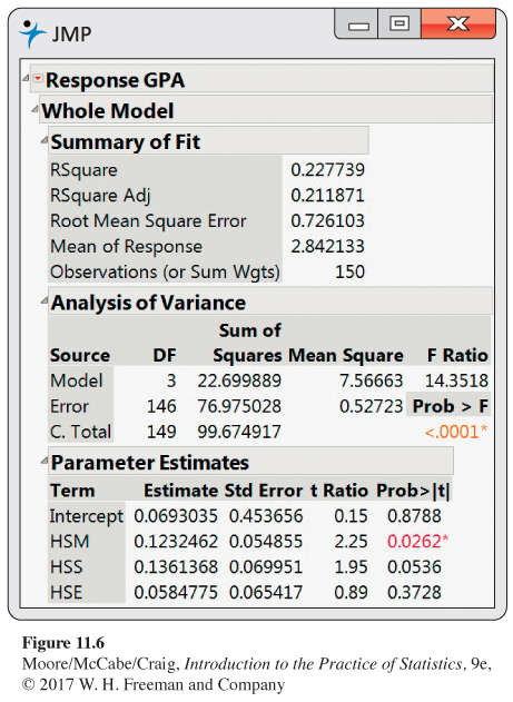
In the fit statistics that precede the ANOVA table, we find that Root MSE is 0.726. This value is the square root of the MSE given in the ANOVA table and is σ, the estimate of the parameter σ of our model. The value of R2 is 0.23. That is, 23% of the observed variation in the GPA scores is explained by linear regression on high school grades.
Although the P-value of the F test is very small, the model does not explain very much of the variation in GPA. Remember, a small P-value does not necessarily tell us that we have a strong predictive relationship, particularly when the sample size is large.
From the Parameter Estimates section of the computer output, we obtain the fitted regression equation
^GPA=0.069+0.123HSM+0.136HSS+0.058HSE
Let’s find the predicted GPA for a student with an A− average in HSM, B+ in HSS, and B in HSE. The explanatory variables are HSM = 9, HSS = 8, and HSE = 7. The predicted GPA is
^GPA=0.069+0.123(9)+0.136(8)+0.058(7)
= 2.67
Recall that the t statistics for testing the regression coefficients are obtained by dividing the estimates by their standard errors. Thus, for the coefficient of HSM, we obtain the t-value given in the output by calculating
t=bSEb=0.123250.05486=2.25
The P-values appear in the last column. Note that these P-values are for the two-
Interpretation of results
The significance tests for the individual regression coefficients seem to contradict the impression obtained by examining the correlations in Figure 11.4. In that display, we see that the correlation between GPA and HSS is 0.44 and the correlation between GPA and HSE is 0.36. The P-values for both of these correlations are < 0.0005. In other words, if we used HSS alone in a regression to predict GPA, or if we used HSE alone, we would obtain statistically significant regression coefficients.
This phenomenon is not unusual in multiple regression analysis. Part of the explanation lies in the correlations between HSM and the other two explanatory variables. These are rather high (at least compared with most other correlations in Figure 11.4). The correlation between HSM and HSS is 0.67 and that between HSM and HSE is 0.49. Thus, when we have a regression model that contains all three high school grades as explanatory variables, there is considerable overlap of the predictive information contained in these variables. This is called collinearitycollinearity or multicollinearitymulticollinearity. In extreme cases, collinearity can cause numerical instabilities that result in very imprecise parameter estimates.
![]()
As mentioned earlier, the significance tests for individual regression coefficients assess the significance of each predictor variable assuming that all other predictors are included in the regression equation. Given that we use a model with HSM and HSS as predictors, the coefficient of HSE is not statistically significant. Similarly, given that we have HSM and HSE in the model, HSS does not have a significant regression coefficient. HSM, however, adds significantly to our ability to predict GPA even after HSS and HSE are already in the model.
Unfortunately, we cannot conclude from this analysis that the pair of explanatory variables HSS and HSE contribute nothing significant to our model for predicting GPA once HSM is in the model. Questions like these require fitting additional models.
The impact of relations among the several explanatory variables on fitting models for the response is the most important new phenomenon encountered in moving from simple linear regression to multiple regression. In this chapter, we can only illustrate some of the many complicated problems that can arise.
residual plots, p. 125
Examining the residuals
As in simple linear regression, we should always examine the residuals as an aid to determining whether the multiple regression model is appropriate for the data. Because there are several explanatory variables, we must examine several residual plots. It is usual to plot the residuals versus the predicted values ˆy and also versus each of the explanatory variables. Look for outliers, influential observations, evidence of a curved (rather than linear) relation, and anything else unusual. We leave the task of making these plots for the case study as an exercise. We find the plots all show more or less random noise above and below the center value of 0.
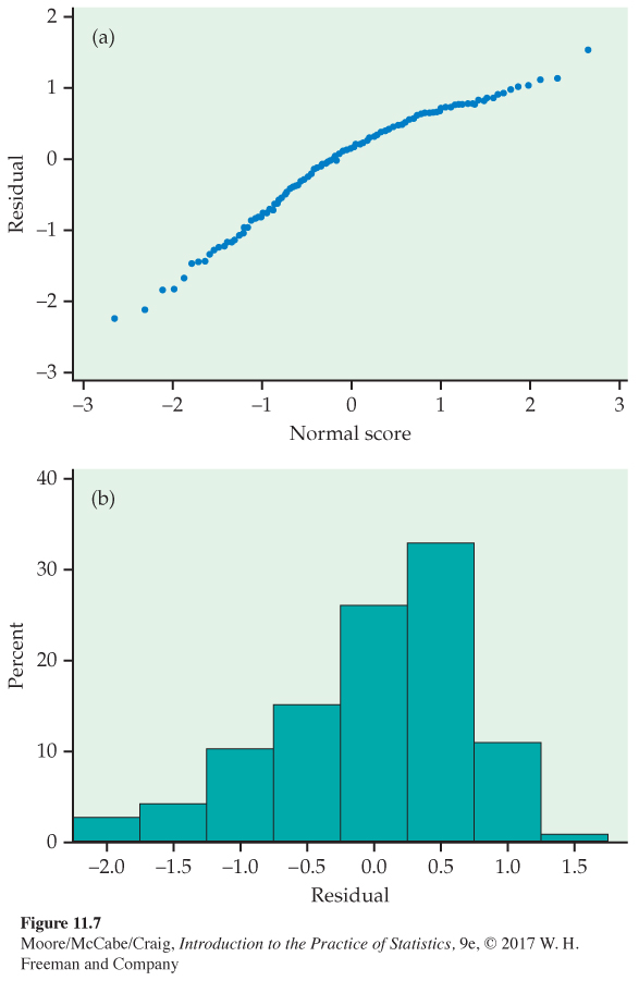
If the deviations ϵ in the model are Normally distributed, the residuals should be Normally distributed. Figure 11.7 presents a Normal quantile plot and histogram of the residuals. Both suggest some skewness (shorter right tail) in the distribution. However, given our large sample size, we do not think this skewness is strong enough to invalidate this analysis.
USE YOUR KNOWLEDGE
Question 11.14
11.14 Residual plots for the GPA analysis. Using a statistical package, fit the linear model with HSM, HSS, and HSE as predictors and obtain the residuals and predicted values. Plot the residuals versus the predicted values, HSM, HSS, and HSE. Are the residuals more or less randomly dispersed around zero? Comment on any unusual patterns.
Refining the model
Because the variable HSE has the largest P-value of the three explanatory variables (see Figure 11.6) and, therefore, appears to contribute the least to our explanation of GPA, we rerun the regression using only HSM and HSS as explanatory variables. The SAS output appears in Figure 11.8. The F statistic indicates that we can reject the null hypothesis that the regression coefficients for the two explanatory variables are both 0. The P-value is still < 0.0001. The value of R2 has dropped very slightly compared with our previous run, from 0.2277 to 0.2235. Thus, dropping HSE from the model resulted in the loss of very little explanatory power.
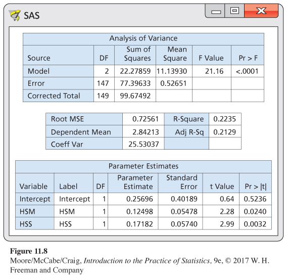
The estimated model standard deviation s (Root MSE in the printout) is nearly identical for the two regressions, another indication that we lose very little when we drop HSE. The t statistics for the individual regression coefficients indicate that HSM is still significant (P = 0.0240), while the statistic for HSS is larger than before (2.99 versus 1.95) and is now statistically significant (P = 0.0032).
Comparison of the fitted equations for the two multiple regression analyses tells us something more about the intricacies of this procedure. For the first run, we have
^GPA=0.069+0.123HSM+0.136HSS+0.058HSE
whereas the second gives us
^GPA=0.257+0.125HSM+0.172HSS
![]()
Eliminating HSE from the model changes the regression coefficients for all the remaining variables and the intercept. This phenomenon occurs quite generally in multiple regression. Individual regression coefficients, their standard errors, and significance tests are meaningful only when interpreted in the context of the other explanatory variables in the model.
Regression on SAT scores
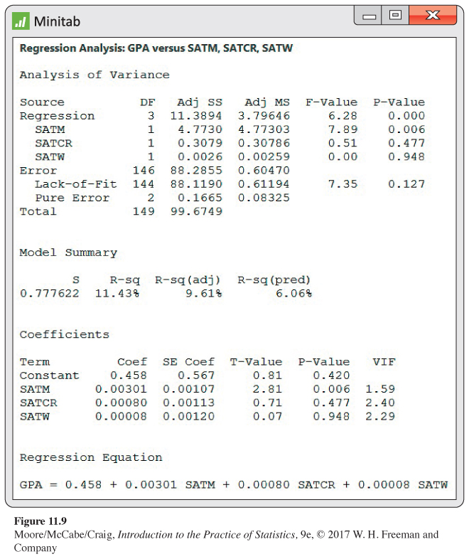
We now turn to the problem of predicting GPA using the three SAT scores. Figure 11.9 gives the Minitab output. The fitted model is
^GPA = 0.458 + 0.00301SATM + 0.00080SATCR + 0.00008SATW
![]()
The degrees of freedom are as expected: 3, 146, and 149. The F statistic is 6.28, with a P-value of < 0.0005. We conclude that the regression coefficients for SATM, SATCR, and SATW are not all 0. Recall that we obtained the P-value < 0.0001 when we used high school grades to predict GPA. Both multiple regression equations are highly significant, but this obscures the fact that the two models have quite different explanatory power. For the SAT regression, R2 = 0.1143, whereas for the high school grades model even with only HSM and HSS (Figure 11.8), we have R2 = 0.2235, a value almost twice as large. Stating that we have a statistically significant result is quite different from saying that an effect is large or important.
Further examination of the output in Figure 11.9 reveals that the coefficient of SATM is significant (t = 2.81, P = 0.006) and that those of SATCR (t = 0.71, P = 0.477) and SATW (t = 0.07, P = 0.948) are not. For a complete analysis, we should carefully examine the residuals. Also, we might want to run the analysis without SATW and the analysis with SATM as the only explanatory variable.
Regression using all variables
We have seen that fitting a model using either the high school grades or the SAT scores results in a highly significant regression equation. The mathematics component of each of these groups of explanatory variables appears to be a key predictor. Comparing the values of R2 for the two models indicates that high school grades are better predictors than SAT scores. Can we get a better prediction equation using all the explanatory variables together in one multiple regression?
To address this question, we run the regression with all six explanatory variables. The output from SAS, Excel, and Minitab appears in Figure 11.10. Although the format and organization of outputs differ among software packages, the basic results that we need are easy to find.
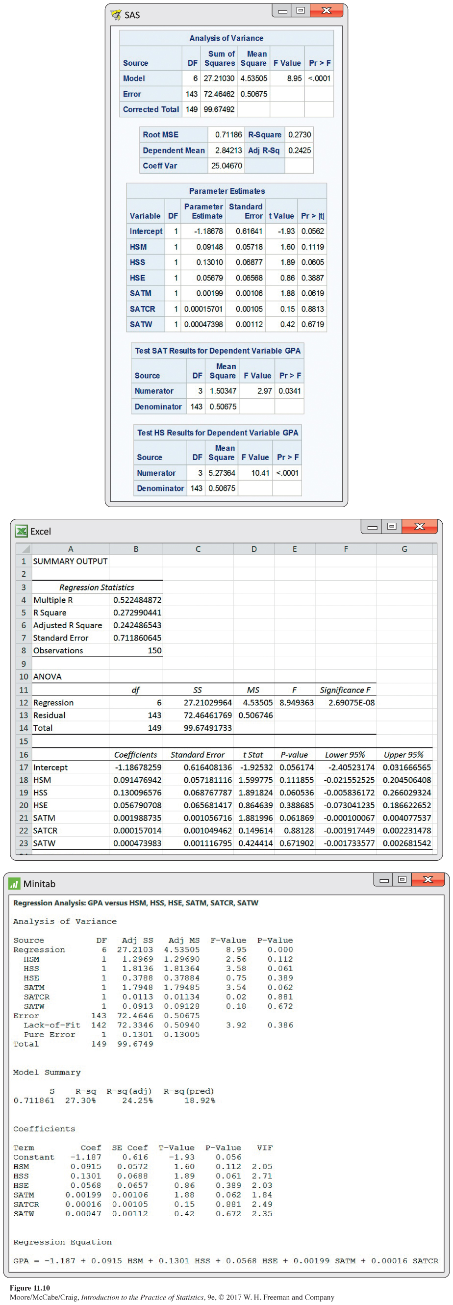
The degrees of freedom are as expected: 6, 143, and 149. The F statistic is 8.95, with a P-value <0.0001, so at least one of our explanatory variables has a nonzero regression coefficient. This result is not surprising, given that we have already seen that HSM and SATM are strong predictors of GPA. The value of R2 is 0.2730, which is about 0.05 higher than the value of 0.2235 that we found for the high school grades regression.
Examination of the t statistics and the associated P-values for the individual regression coefficients reveals a surprising result. None of the variables are significant! At first, this result may appear to contradict the ANOVA results. How can the model explain more than 27% of the variation and have t tests that suggest none of the variables make a significant contribution?
Once again, it is important to understand that these t tests assess the contribution of each variable when it is added to a model that already has the other five explanatory variables. This result does not necessarily mean that the regression coefficients for the six explanatory variables are all 0. It simply means that the contribution of each variable overlaps considerably with the contribution of the other five variables already in the model.
When a model has a large number of insignificant variables, it is common to refine the model. This is often termed model selectionmodel selection. We prefer smaller models to larger models because they are easier to work with and understand. However, given the many complications that can arise in multiple regression, there is no universal “best’’ approach to refine a model. There is also no guarantee that there is just one acceptable refined model.
Many statistical software packages now provide the capability of summarizing all possible models from a set of p variables. We suggest using this capability when possible to reduce the number of candidate models (for example, there are a total of 63 models when p = 6) and then carefully studying the remaining models before making a decision as to a best model or set of best models. If in doubt, consult an expert.
For example, Figure 11.11 contains the output from the SAS commands
proc reg;
model GPA = HSM HSS HSE SATM SATCR SATW/selection=rsquare mse best=2;
run;
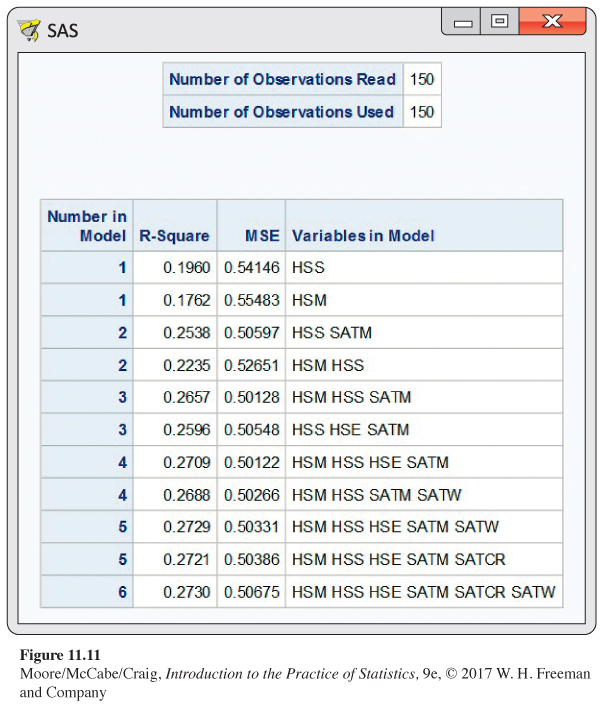
It shows the two best models in terms of highest R2, when the number of explanatory variables in the model are p = 1 through p = 6. A list like this can be very helpful in reducing the number of models to consider. In this case, there’s very little difference in R2 once the model has at least three explanatory variables, so we might consider further studying just the four models listed with p = 3 or p = 4.
The list also contains the estimated model variance (MSE). Finding a model (or models) that minimizes this quantity is another model selection approach. It is equivalent to choosing a model based on adjusted R2adjusted R2. Unlike R2, the adjusted R2 and MSE take into account the number of parameters in the model and thus penalize larger models. In Figure 11.11, we see a model with p = 3 and a model with p = 4 have the two smallest MSEs. Pending an examination of the residuals, these are the two best refined models based on this selection method.
Test for a collection of regression coefficients
Many statistical software packages also provide the capability for testing whether a collection of regression coefficients in a multiple regression model are all 0. We use this approach to address two interesting questions about our data set. We did not discuss such tests in the outline that opened this section, but the basic idea is quite simple and is discussed in Exercise 11.20 (page 635).
In the context of the multiple regression model with all six predictors, we ask first whether or not the coefficients for the three SAT scores are all 0. In other words, do the SAT scores add any significant predictive information to that already contained in the high school grades? To be fair, we also ask the complementary question: do the high school grades add any significant predictive information to that already contained in the SAT scores?
The answers are given in the last two parts of the SAS output in Figure 11.10 (page 628). For the first test, we see that F = 2.97. Under the null hypothesis that the three SAT coefficients are 0, this statistic has an F(3,143) distribution and the P-value is 0.0341. We conclude that the SAT scores (as a group) are significant predictors of GPA in a regression that already contains the high school scores as predictor variables. This means that we cannot just focus on refined models that involve the high school grades. Both high school grades and SAT scores appear to contribute to our explanation of GPA.
The test statistic for the three high school grade variables is F = 10.41. Under the null hypothesis that these three regression coefficients are 0, the statistic has an F(3,143) distribution and the P-value is <0.0001. Again, this means that high school grades contain useful information for predicting GPA that is not contained in the SAT scores.
BEYOND THE BASICS
Multiple Logistic Regression
Many studies have yes/no or success/failure response variables. A surgery patient lives or dies; a consumer does or does not purchase a product after viewing an advertisement. Because the response variable in a multiple regression is assumed to have a Normal distribution, this methodology is not suitable for predicting such responses. However, there are models that apply the ideas of regression to response variables with only two possible outcomes.
One type of model that can be used is called logistic regressionlogistic regression. We think in terms of a binomial model for the two possible values of the response variable and use one or more explanatory variables to explain the probability of success. Details are more complicated than those for multiple regression and are given in Chapter 14. However, the fundamental ideas are very much the same. Here is an example.
EXAMPLE 11.2

Tipping behavior in Canada. The Consumer Report on Eating Share Trends (CREST) contains data spanning all provinces of Canada and details away-
The model consisted of more than 25 explanatory variables, grouped as “control’’ variables and “stereotype-
chi-
Similar to the F test in multiple regression, there is a chi-
Interpretation of the coefficients is a little more difficult in multiple logistic regression because of the form of the model. For example, the high-
log(p1−p) = β0 + β1x1 + β2x2 + … + β6x6
The expression p/(1 − p) is the oddsodds that the tip was above 20%. Logistic regression models the “log odds’’ as a linear combination of the explanatory variables. Positive coefficients are associated with a higher probability that the tip is high. These coefficients are often transformed back (eβj) to the odds scale, giving us an odds ratioodds ratio. An odds ratio greater than 1 is associated with a higher probability that the tip is high. Here is the table of odds ratios reported in the article for the high-
| Explanatory variable | Odds ratio |
|---|---|
| Senior adult | 0.7420* |
| Sunday | 0.9970 |
| English as second language | 0.7360* |
| French- |
0.7840* |
| Alcoholic drinks | 1.1250* |
| Lone male | 1.0220* |
The starred values were significant at the 0.01 level. We see that the probability of a high tip is reduced (odds ratio less than 1) when the diner is over 65 years old, speaks English as a second language, and is a French-