13.2 13.2 Inference for Two-Way ANOVA
When you complete this section, you will be able to:
• Construct the two-
way ANOVA table in terms of sources and degrees of freedom. • Summarize what the ANOVA table F tests can tell you about main effects and interactions and what they cannot without further analysis.
• Interpret statistical software ANOVA output for a two-
way ANOVA .• Use residual plots and sample statistics to check the assumptions of the two-
way ANOVA model.
Inference for two-
The ANOVA table for two-
Two-
SST = SSA + SSB + SSAB + SSE
DFT = DFA + DFB + DFAB + DFE
The sums of squares are always calculated in practice by statistical software. When the nij are not all equal, there are different ways to calculate the sums of squares, and some can give sums of squares that do not add. The degrees of freedom, on the other hand, will always add.
![]()
From each sum of squares and its degrees of freedom we find the mean square in the usual way:
mean square=sum of squaresdegrees of freedom
The significance of each of the main effects and the interaction is assessed by an F statistic that compares the variation due to the effect of interest with the within-
| Source | Degrees of freedom | Sum of squares | Mean square | F |
|---|---|---|---|---|
| A | I − 1 | SSA | SSA/DFA | MSA/MSE |
| B | J − 1 | SSB | SSB/DFB | MSB/MSE |
| AB | (I − 1) (J − 1) | SSAB | SSAB/DFAB | MSAB/MSE |
| Error | N−IJ | SSE | SSE/DFE | |
| Total | N − 1 | SST |
![]()
There are three null hypotheses in two-
SIGNIFICANCE TESTS IN TWO-
To test the main effect of A, use the F statistic
FA=MSAMSE
To test the main effect of B, use the F statistic
FB=MSBMSE
To test the interaction of A and B, use the F statistic
FAB=MSABMSE
The P-value is the probability that a random variable having an F distribution with numerator degrees of freedom corresponding to the effect and denominator degrees of freedom equal to DFE is greater than or equal to the calculated F statistic.
The following example illustrates how to do a two-
EXAMPLE 13.8
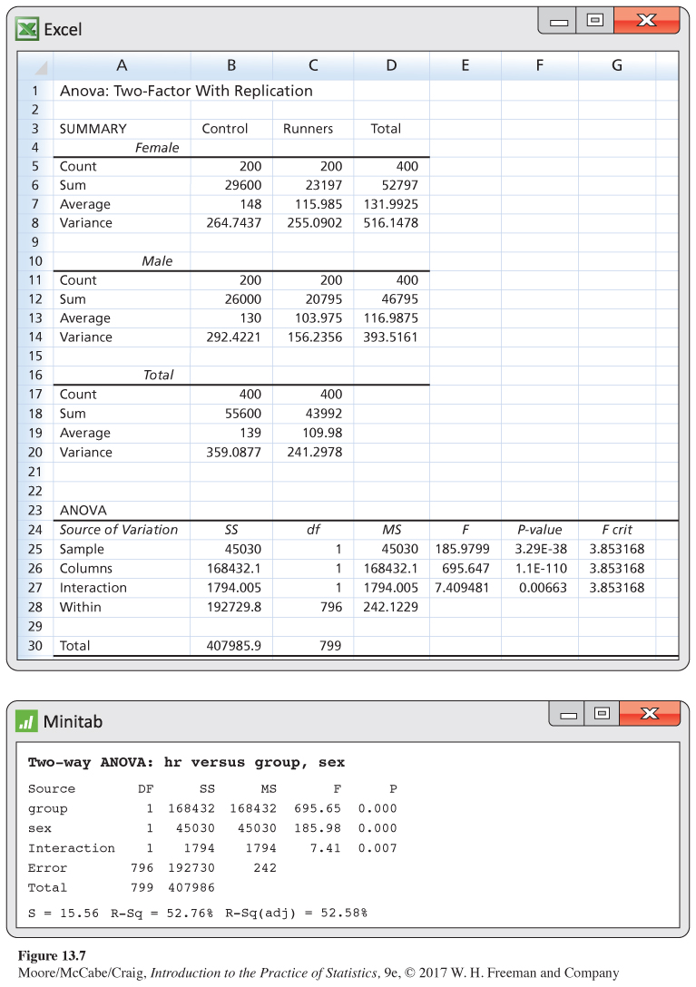
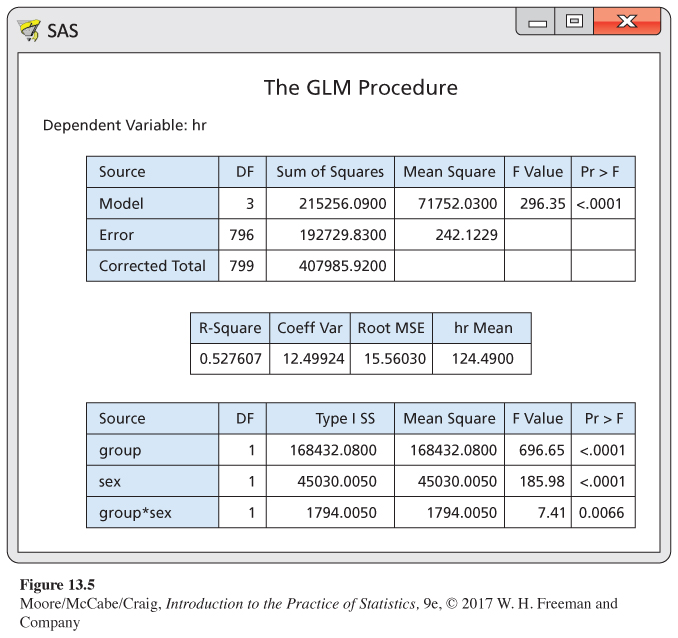
A study of cardiovascular risk factors. A study of cardiovascular risk factors compared runners who averaged at least 15 miles per week with a control group described as “generally sedentary.’’ Both men and women were included in the study.6 The design is a 2 × 2 ANOVA with the factors group and sex. There were 200 subjects in each of the four combinations. One of the variables measured was the heart rate after six minutes of exercise on a treadmill. SAS computer analysis produced the outputs in Figure 13.4 and Figure 13.5.
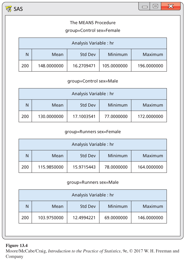
We begin with the usual preliminary examination. From Figure 13.4, we see that the ratio of the largest to the smallest standard deviation is less than 2. Therefore, we are not concerned about violating the assumption of equal population standard deviations. Normal quantile plots (not shown) do not reveal any outliers, and the data appear to be reasonably Normal.
![]()
The ANOVA table at the top of the output in Figure 13.5 is, in effect, a one-
The sums of squares for the group and sex main effects and the group-
Because the degrees of freedom are all 1 for the main effects and the interaction, the mean squares are the same as the sums of squares. The F statistics for the three effects appear in the column labeled “F Value,’’ and the P-values are under the heading “Pr > F.’’ For the group main effect, we verify the calculation of F as follows:
F=MSGMSE=168,432242.12=695.65
All three effects are statistically significant. The group effect has the largest F, followed by the sex effect and then the group-
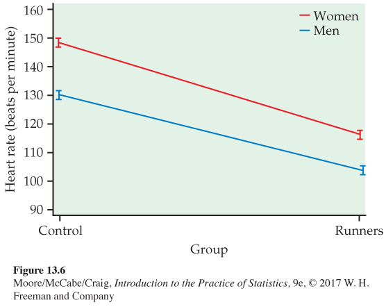
The significance of the main effect for sex is due to the fact that the females have higher heart rates than the men in both groups. The differences are not as large as those for the group effect, and this is reflected in the smaller value of the F statistic.
The analysis indicates that a complete description of the average heart rates requires consideration of the interaction in addition to the main effects. The two lines in the plot are not parallel. This interaction can be described in two ways. The female-
Two-