SECTION 1.4 EXERCISES
For Exercises 1.93 and 1.94, see page 59; for Exercises 1.95 and 1.96, see page 60; for Exercises 1.97 and 1.98, see page 64; and for Exercises 1.99 and 1.100, see page 66.
Question 1.101
1.101 Means and medians.
(a) Sketch a symmetric distribution that is not Normal. Mark the location of the mean and the median.
(b) Sketch a distribution that is skewed to the left. Mark the location of the mean and the median.
Question 1.102
1.102 The effect of changing the standard deviation.
(a) Sketch a Normal curve that has mean 30 and standard deviation 8.
(b) On the same x axis, sketch a Normal curve that has mean 30 and standard deviation 12.
(c) How does the Normal curve change when the standard deviation is varied but the mean stays the same?
Question 1.103
1.103 The effect of changing the mean.
(a) Sketch a Normal curve that has mean 30 and standard deviation 8.
(b) On the same x axis, sketch a Normal curve that has mean 40 and standard deviation 8.
(c) How does the Normal curve change when the mean is varied but the standard deviation stays the same?
Question 1.104
1.104 NAEP music scores. In Exercise 1.93 (page 59) we examined the distribution of NAEP scores for the 12th-grade reading skills assessment. For eighth-grade students, the average music score is approximately Normal with mean 150 and standard deviation 35.
(a) Sketch this Normal distribution.
(b) Make a table that includes values of the scores corresponding to plus or minus one, two, and three standard deviations from the mean. Mark these points on your sketch along with the mean.
(c) Apply the 68–95–99.7 rule to this distribution. Give the ranges of reading score values that are within one, two, and three standard deviations of the mean.
Question 1.105
1.105 NAEP U.S. history scores. Refer to the previous exercise. The scores for 12th-grade students on the U.S. history assessment are approximately N(288,32) Answer the questions in the previous exercise for this assessment.
1.105 (b)–(c) The following table indicates the desired ranges.
| Low | High | |
|---|---|---|
| 68% | 256 | 320 |
| 95% | 224 | 352 |
| 99.7% | 192 | 384 |
Question 1.106
1.106 Standardize some NAEP music scores. The NAEP music assessment scores for eighth-grade students are approximately N(150,35). Find z-scores by standardizing the following scores: 150, 140, 100, 180, 230.
Question 1.107
1.107 Compute the percentile scores. Refer to the previous exercise. When scores such as the NAEP assessment scores are reported for individual students, the actual values of the scores are not particularly meaningful. Usually, they are transformed into percentile scores. The percentile score is the proportion of students who would score less than or equal to the score for the individual student. Compute the percentile scores for the five scores in the previous exercise. State whether you used software or Table A for these computations.
1.107
| Value | Percentile (Table A) | Percentile (Software) |
|---|---|---|
| 150 | 50 | 50 |
| 140 | 38.6 | 38.8 |
| 100 | 7.6 | 7.7 |
| 180 | 80.5 | 80.4 |
| 230 | 98.9 | 98.9 |
Question 1.108
![]() 1.108 Are the NAEP U.S. history scores approximately Normal? In Exercise 1.105, we assumed that the NAEP U.S history scores for 12th-grade students are approximately Normal with the reported mean and standard deviation, N(288,32). Let’s check that assumption. In addition to means and standard deviations, you can find selected percentiles for the NAEP assessments (see previous exercise). For the 12th-grade U.S. history scores, the following percentiles are reported:
1.108 Are the NAEP U.S. history scores approximately Normal? In Exercise 1.105, we assumed that the NAEP U.S history scores for 12th-grade students are approximately Normal with the reported mean and standard deviation, N(288,32). Let’s check that assumption. In addition to means and standard deviations, you can find selected percentiles for the NAEP assessments (see previous exercise). For the 12th-grade U.S. history scores, the following percentiles are reported:
| Percentile | Score |
|---|---|
| 10% | 246 |
| 25% | 276 |
| 50% | 290 |
| 75% | 311 |
| 90% | 328 |
Use these percentiles to assess whether or not the NAEP U.S History scores for 12th-grade students are approximately Normal. Write a short report describing your methods and conclusions.
Question 1.109
![]() 1.109 Are the NAEP mathematics scores approximately Normal? Refer to the previous exercise. For the NAEP mathematics scores for 12th-graders, the mean is 153 and the standard deviation is 34. Here are the reported percentiles:
1.109 Are the NAEP mathematics scores approximately Normal? Refer to the previous exercise. For the NAEP mathematics scores for 12th-graders, the mean is 153 and the standard deviation is 34. Here are the reported percentiles:
| Percentile | Score |
|---|---|
| 10% | 110 |
| 25% | 130 |
| 50% | 154 |
| 75% | 177 |
| 90% | 197 |
Is the N(153,34) distribution a good approximation for the NAEP mathematics scores? Write a short report describing your methods and conclusions.
1.109 Using the N(153, 34) distribution, we find the values corresponding to the given percentiles as given here (using Table A). The actual scores are very close to the percentiles of the Normal distribution; we can conclude these scores are at least approximately Normal.
| Percentile | Score | Score with N(153, 34) |
|---|---|---|
| 10% | 110 | 109 |
| 25% | 130 | 130 |
| 50% | 154 | 153 |
| 75% | 177 | 176 |
| 90% | 197 | 197 |
Question 1.110
1.110 Do women talk more? Conventional wisdom suggests that women are more talkative than men. One study designed to examine this stereotype collected data on the speech of 42 women and 37 men in the United States.35
(a) The mean number of words spoken per day by the women was 14,297 with a standard deviation of 6441. Use the 68–95–99.7 rule to describe this distribution.
(b) Do you think that applying the rule in this situation is reasonable? Explain your answer.
(c) The men averaged 14,060 words per day with a standard deviation of 9056. Answer the questions in parts (a) and (b) for the men.
(d) Do you think that the data support the conventional wisdom? Explain your answer. Note that in Section 7.2 we will learn formal statistical methods to answer this type of question.
Question 1.111
1.111 Data from Mexico. Refer to the previous exercise. A similar study in Mexico was conducted with 31 women and 20 men. The women averaged 14,704 words per day with a standard deviation of 6215. For men the mean was 15,022 and the standard deviation was 7864.
(a) Answer the questions from the previous exercise for the Mexican study.
(b) The means for both men and women are higher for the Mexican study than for the U.S. study. What conclusions can you draw from this observation?
1.111 (a) Ranges are shown in the following table. In both cases, some of the lower limits are negative, which does not make sense; this happens because the women’s distribution is skewed and the men’s distribution has an outlier. Contrary to the conventional wisdom, the men’s mean is slightly higher, although the outlier is at least partly responsible for that. (b) The means suggest that Mexican men and women tend to speak more than people of the same sex from the United States.
| Women | Men | |
|---|---|---|
| 68% | 8489 to 20,919 | 7158 to 22,886 |
| 95% | 2274 to 27,134 | − 706 to 30,750 |
| 99.7% | − 3941 to 33,349 | − 8570 to 38,614 |
Question 1.112
1.112 A uniform distribution. If you ask a computer to generate “random numbers” between 0 and 1, you will get observations from a uniform distribution. Figure 1.33 graphs the density curve for a uniform distribution. Use areas under this density curve to answer the following questions.
(a) Why is the total area under this curve equal to 1?
(b) What proportion of the observations lie above 0.44?
(c) What proportion of the observations lie between 0.44 and 0.70?
Question 1.113
1.113 Use a different range for the uniform distribution. Many random number generators allow users to specify the range of the random numbers to be produced. Suppose that you specify that the outcomes are to be distributed uniformly between 0 and 4. Then the density curve of the outcomes has constant height between 0 and 4, and height 0 elsewhere.
(a) What is the height of the density curve between 0 and 4? Draw a graph of the density curve.
(b) Use your graph from part (a) and the fact that areas under the curve are proportions of outcomes to find the proportion of outcomes that are more than 1.
(c) Find the proportion of outcomes that lie between 1.5 and 2.5.
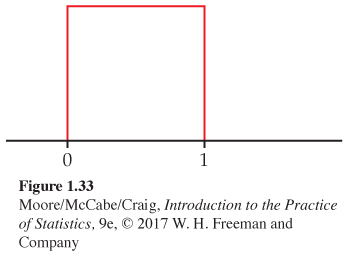
1.113 (a) 0.25. (b) 0.75. (c) 0.25.
Question 1.114
1.114 Find the mean, the median, and the quartiles. What are the mean and the median of the uniform distribution in Figure 1.33? What are the quartiles?
Question 1.115
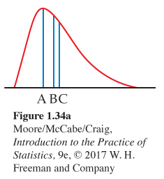
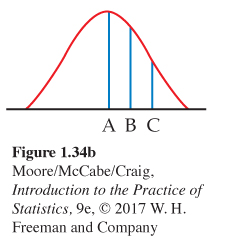
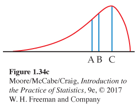
1.115 Three density curves. Figure 1.34 displays three density curves, each with three points marked on it. At which of these points on each curve do the mean and the median fall?
1.115 (a) The mean is at point C; the median is at point B. (b) The mean and median are both at point A. (c) The mean is at point A; the median is at point B.
Question 1.116
![]() 1.116 Use the Normal Curve applet. Use the Normal Curve applet for the standard Normal distribution to say how many standard deviations above and below the mean the quartiles of any Normal distribution lie.
1.116 Use the Normal Curve applet. Use the Normal Curve applet for the standard Normal distribution to say how many standard deviations above and below the mean the quartiles of any Normal distribution lie.
Question 1.117
![]() 1.117 Use the Normal Curve applet.
The 68–95–99.7 rule for Normal distributions is a useful approximation. You can use the Normal Curve applet on the text website to see how accurate the rule is. Drag one flag across the other so that the applet shows the area under the curve between the two flags.
1.117 Use the Normal Curve applet.
The 68–95–99.7 rule for Normal distributions is a useful approximation. You can use the Normal Curve applet on the text website to see how accurate the rule is. Drag one flag across the other so that the applet shows the area under the curve between the two flags.
(a) Place the flags one standard deviation on either side of the mean. What is the area between these two values? What does the 68–95–99.7 rule say this area is?
(b) Repeat for locations two and three standard deviations on either side of the mean. Again compare the 68–95–99.7 rule with the area given by the applet.
1.117 (a) The applet shows an area of 0.6826 between − 1.000 and 1.000, while the 68 − 95 − 99.7 rule rounds this to 0.68. (b) Between − 2.000 and 2.000, the applet reports 0.9544 (compared to the rounded 0.95 from the 68 − 95 − 99.7 rule). Between − 3.000 and 3.000, the applet reports 0.9974 (compared to the rounded 0.997).
Question 1.118
1.118 Find some proportions. Using either Table A or your calculator or software, find the proportion of observations from a standard Normal distribution that satisfies each of the following statements. In each case, sketch a standard Normal curve and shade the area under the curve that is the answer to the question.
(a) Z > 1.75
(b) Z < 1.75
(c) Z > −0.80
(d) −0.80 < Z < 1.75
Question 1.119
1.119 Find more proportions. Using either Table A or your calculator or software, find the proportion of observations from a standard Normal distribution for each of the following events. In each case, sketch a standard Normal curve and shade the area representing the proportion.
(a) Z ≤ −1.4
(b) Z ≥ −1.4
(c) Z > 2.0
(d) −1.4 < Z < 2.0
1.119 (a) 0.0808. (b) 0.9192. (c) 0.0228. (d) 0.8964.
Question 1.120
1.120 Find some values of z. Find the value z of a standard Normal variable Z that satisfies each of the following conditions. (If you use Table A, report the value of z that comes closest to satisfying the condition.) In each case, sketch a standard Normal curve with your value of z marked on the axis.
(a) 38% of the observations fall below z
(b) 70% of the observations fall above z
Question 1.121
1.121 Find more values of z. The variable Z has a standard Normal distribution.
(a) Find the number z that has cumulative proportion 0.88.
(b) Find the number z such that the event Z > z has proportion 0.12.
1.121 (a) z = 1.17 or 1.18. (b) z = 1.17 or 1.18.
Question 1.122
1.122 Find some values of z. The Wechsler Adult Intelligence Scale (WAIS) is the most common IQ test. The scale of scores is set separately for each age group, and the scores are approximately Normal with mean 100 and standard deviation 15. People with WAIS scores below 70 are considered developmentally disabled when, for example, applying for Social Security disability benefits. What percent of adults are developmentally disabled by this criterion?
Question 1.123
1.123 High IQ scores. The Wechsler Adult Intelligence Scale (WAIS) is the most common IQ test. The scale of scores is set separately for each age group, and the scores are approximately Normal with mean 100 and standard deviation 15. The organization MENSA, which calls itself “the high-IQ society,” requires a WAIS score of 130 or higher for membership. What percent of adults would qualify for membership?
There are two major tests of readiness for college, the ACT and the SAT. ACT scores are reported on a scale from 1 to 36. The distribution of ACT scores is approximately Normal with mean μ = 21.5 and standard deviation σ = 5.4. SAT scores are reported on a scale from 600 to 2400. The distribution of SAT scores is approximately Normal with mean μ = 1498 and standard deviation σ = 316. Exercises 1.124 through 1.133 are based on this information.
1.123 z = 2. From Table A, 2.28% qualify for membership.
Question 1.124
1.124 Compare an SAT score with an ACT score. Jessica scores 1830 on the SAT. Ashley scores 27 on the ACT. Assuming that both tests measure the same thing, who has the higher score? Report the z-scores for both students.
Question 1.125
1.125 Make another comparison. Joshua scores 16 on the ACT. Anthony scores 1050 on the SAT. Assuming that both tests measure the same thing, who has the higher score? Report the z-scores for both students.
1.125 For Joshua, z = − 1.02. For Anthony, z = − 1.42. Joshua has the higher standardized score.
Question 1.126
1.126 Find the ACT equivalent. Jorge scores 2090 on the SAT. Assuming that both tests measure the same thing, what score on the ACT is equivalent to Jorge’s SAT score?
Question 1.127
1.127 Find the SAT equivalent. Alyssa scores 30 on the ACT. Assuming that both tests measure the same thing, what score on the SAT is equivalent to Alyssa’s ACT score?
1.127 z = 1.57. The equivalent SAT score is 1994.12.
Question 1.128
1.128 Find an SAT percentile. Reports on a student’s ACT or SAT results usually give the percentile as well as the actual score. The percentile is just the cumulative proportion stated as a percent: the percent of all scores that were lower than or equal to this one. Renee scores 2050 on the SAT. What is her percentile?
Question 1.129
1.129 Find an ACT percentile. Reports on a student’s ACT or SAT results usually give the percentile as well as the actual score. The percentile is just the cumulative proportion stated as a percent: the percent of all scores that were lower than or equal to this one. Joshua scores 19 on the ACT. What is his percentile?
1.129 z = − 0.46. From Table A we get 0.3228, so about the 32nd percentile.
Question 1.130
1.130 How high is the top 12%? What SAT scores make up the top 12% of all scores?
Question 1.131
1.131 How low is the bottom 12%? What SAT scores make up the bottom 12% of all scores?
1.131 Scores 1125.12 and lower make up the bottom 12% of all scores.
Question 1.132
1.132 Find the ACT quintiles. The quintiles of any distribution are the values with cumulative proportions 0.20, 0.40, 0.60, and 0.80. What are the quintiles of the distribution of ACT scores?
Question 1.133
1.133 Find the SAT quartiles. The quartiles of any distribution are the values with cumulative proportions 0.25 and 0.75. What are the quartiles of the distribution of SAT scores?
1.133 From Table A, the quartiles have z-scores of − 0.675, 0, and 0.675. Using 1498 + 316(z) yields scores of 1285, 1498, and 1711 (rounded to the nearest integer).
Question 1.134
1.134 Do you have enough “good cholesterol?” High-density lipoprotein (HDL) is sometimes called the “good cholesterol” because low values are associated with a higher risk of heart disease. According to the American Heart Association, people over the age of 20 years should have at least 40 milligrams per deciliter (mg/dl) of HDL cholesterol.36 U.S. women aged 20 and over have a mean HDL of 55 mg/dl with a standard deviation of 15.5 mg/dl. Assume that the distribution is Normal.
(a) What percent of women have low values of HDL (40 mg/dl or less)?
(b) HDL levels of 60 mg/dl and higher are believed to protect people from heart disease. What percent of women have protective levels of HDL?
(c) Women with more than 40 mg/dl but less than 60 mg/dl of HDL are in the intermediate range, neither very good or very bad. What proportion are in this category?
Question 1.135
1.135 Men and HDL cholesterol. HDL cholesterol levels for men have a mean of 46 mg/dl with a standard deviation of 13.6 mg/dl. Answer the questions given in the previous exercise for the population of men.
1.135 (a) z = − 0.44. From Table A, 33% of men have low values of HDL. (Software gives 32.95%.) (b) z = 1.03. From Table A, 15.15% of men have protective levels of HDL. (Software gives 15.16%.) (c) 51.85% of men are in the intermediate range for HDL. (Software gives 0.5188.)
Question 1.136
1.136 Diagnosing osteoporosis. Osteoporosis is a condition in which the bones become brittle due to loss of minerals. To diagnose osteoporosis, an elaborate apparatus measures bone mineral density (BMD). BMD is usually reported in standardized form. The standardization is based on a population of healthy young adults. The World Health Organization (WHO) criterion for osteoporosis is a BMD 2.5 standard deviations below the mean for young adults. BMD measurements in a population of people similar in age and sex roughly follow a Normal distribution.
(a) What percent of healthy young adults have osteoporosis by the WHO criterion?
(b) Women aged 70 to 79 are of course not young adults. The mean BMD in this age is about −2 on the standard scale for young adults. Suppose that the standard deviation is the same as for young adults. What percent of this older population has osteoporosis?
Question 1.137
1.137 Deciles of Normal distributions. The deciles of any distribution are the 10th, 20th, . . ., 90th percentiles. The first and last deciles are the 10th and 90th percentiles, respectively.
(a) What are the first and last deciles of the standard Normal distribution?
(b) The weights of 9-ounce potato chip bags are approximately Normal with mean 9.12 ounces and standard deviation 0.15 ounce. What are the first and last deciles of this distribution?
1.137 (a) The first and last deciles for a standard Normal distribution are ± 1.2816. (b) For a N(9.12, 0.15) distribution, the first and last deciles are 8.93 and 9.31 ounces.
Question 1.138
![]() 1.138 Quartiles for Normal distributions. The quartiles of any distribution are the values with cumulative proportions 0.25 and 0.75.
1.138 Quartiles for Normal distributions. The quartiles of any distribution are the values with cumulative proportions 0.25 and 0.75.
(a) What are the quartiles of the standard Normal distribution?
(b) Using your numerical values from part (a), write an equation that gives the quartiles of the N(μ, σ) distribution in terms of μ and σ.
Question 1.139
![]() 1.139 IQR for Normal distributions. Continue your work from the previous exercise. The interquartile range IQR is the distance between the first and third quartiles of a distribution.
1.139 IQR for Normal distributions. Continue your work from the previous exercise. The interquartile range IQR is the distance between the first and third quartiles of a distribution.
(a) What is the value of the IQR for the standard Normal distribution?
(b) There is a constant c such that IQR − cσ for any Normal distribution N(μ, σ). What is the value of c?
1.139 (a) As the quartiles for a standard Normal distribution are ± 0.6745, we have IQR = 1.3490. (b) c = 1.3490.
Question 1.140
![]() 1.140 Outliers for Normal distributions. Continue your work from the previous two exercises. The percent of the observations that are suspected outliers according to the 1.5 × IQR rule is the same for any Normal distribution. What is this percent?
1.140 Outliers for Normal distributions. Continue your work from the previous two exercises. The percent of the observations that are suspected outliers according to the 1.5 × IQR rule is the same for any Normal distribution. What is this percent?
Question 1.141
1.141 Deciles of HDL cholesterol. The deciles of any distribution are the 10th, 20th, . . . , 90th percentiles. Refer to Exercise 1.134 where we assumed that the distribution of HDL cholesterol in U.S. women aged 20 and over is Normal with mean 55 mg/dl and standard deviation 15.5 mg/dl. Find the deciles for this distribution.
1.141 The deciles are shown here.
| Percentile | 10% | 20% | 30% | 40% | 50% |
| HDL level | 35.2 | 42.0 | 46.9 | 51.1 | 55 |
| Percentile | 60% | 70% | 80% | 90% | |
| HDL level | 58.9 | 63.1 | 68.0 | 74.8 |
Question 1.142
1.142 Longleaf pine trees. Exercise 1.88 (page 50) gives the diameter at breast height (DBH) for 40 longleaf pine trees from the Wade Tract in Thomas County, Georgia. Make a Normal quantile plot for these data and write a short paragraph interpreting what it describes.
Question 1.143
1.143 Potassium from potatoes. Refer to Exercise 1.30 (page 24) where you used a stemplot to examine the potassium absorption of a group of 27 adults who ate a controlled diet that included 40 mEq of potassium from potatoes for five days. In Exercise 1.61 (page 47), you compared the stemplot, the histogram, and the boxplot as graphical summaries of this distribution.
(a) Generate these three graphical summaries.
(b) Make a Normal quantile plot and interpret it.
1.143 (b) The data are roughly Normal, but there is one potential high outlier.
Question 1.144
1.144 Potassium from a supplement. Refer to Exercise 1.31 (page 24) where you used a stemplot to examine where you examined the potassium absorption of a group of 29 adults who ate a controlled diet that included 40 mEq of potassium from a supplement for five days. In Exercise 1.62 (page 47), you compared the stemplot, the histogram, and the boxplot as graphical summaries of this distribution.
(a) Generate these three graphical summaries.
(b) Make a Normal quantile plot and interpret it.