2.5 2.4 Least-Squares Regression
When you complete this section, you will be able to:
• Draw a straight line on a scatterplot of a set of data, given the equation of the line.
• Predict a value of the response variable y for a given value of the explanatory variable x using a regression equation.
• Explain the meaning of the term least squares.
• Calculate the equation of a least-squares regression line from the means and standard deviations of the explanatory and response variables and their correlation.
• Read the output of statistical software to find the equation of the least-squares regression line and the value of r2.
• Explain the meaning of r2 in the regression setting.
Correlation measures the direction and strength of the linear (straight-line) relationship between two quantitative variables. If a scatterplot shows a linear relationship, we would like to summarize this overall pattern by drawing a line on the scatterplot. A regression line summarizes the relationship between two variables, but only in a specific setting: when one of the variables helps explain or predict the other. That is, regression describes a relationship between an explanatory variable and a response variable.
REGRESSION LINE
A regression line is a straight line that describes how a response variable y changes as an explanatory variable x changes. We often use a regression line to predict the value of y for a given value of x. Regression, unlike correlation, requires that we have an explanatory variable and a response variable.
EXAMPLE 2.19
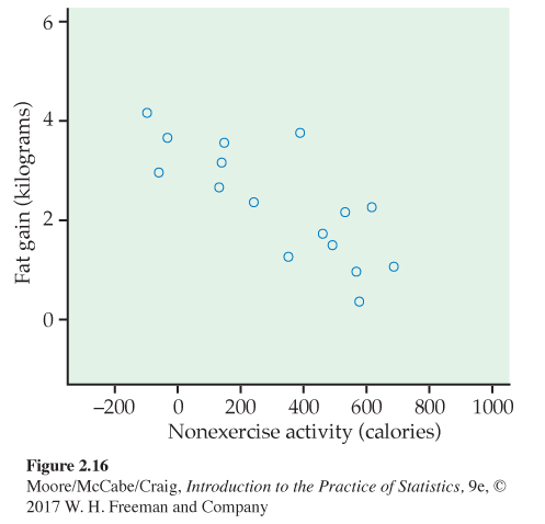
Fidgeting and fat gain. Does fidgeting keep you slim? Some people don’t gain weight even when they overeat. Perhaps fidgeting and other “nonexercise activity” (NEA) explains why—the body might spontaneously increase nonexercise activity when fed more. Researchers deliberately overfed 16 healthy young adults for eight weeks. They measured fat gain (in kilograms) and, as an explanatory variable, increase in energy use (in calories) from activity other than deliberate exercise—fidgeting, daily living, and the like. Here are the data:17
| NEA increase (cal) | −94 | −57 | −29 | 135 | 143 | 151 | 245 | 355 |
| Fat gain (kg) | 4.2 | 3.0 | 3.7 | 2.7 | 3.2 | 3.6 | 2.4 | 1.3 |
| NEA increase (cal) | 392 | 473 | 486 | 535 | 571 | 580 | 620 | 690 |
| Fat gain (kg) | 3.8 | 1.7 | 1.6 | 2.2 | 1.0 | 0.4 | 2.3 | 1.1 |
Figure 2.16 is a scatterplot of these data. The plot shows a moderately strong negative linear association with no outliers. The correlation is r = −0.7786. People with larger increases in nonexercise activity do indeed gain less fat. A line drawn through the points will describe the overall pattern well.
Fitting a line to data
When a scatterplot displays a linear pattern, we can describe the overall pattern by drawing a straight line through the points. Of course, no straight line passes exactly through all the points. Fitting a linefitting a line to data means drawing a line that comes as close as possible to the points. The equation of a line fitted to the data gives a concise description of the relationship between the response variable y and the explanatory variable x. It is the numerical summary that supports the scatterplot, our graphical summary.
STRAIGHT LINES
Suppose that y is a response variable (plotted on the vertical axis) and x is an explanatory variable (plotted on the horizontal axis). A straight line relating y to x has an equation of the form
y = b0 + b1x
In this equation, b1 is the slope, the amount by which y changes when x increases by one unit. The number b0 is the intercept, the value of y when x = 0.
In practice, we will use software to obtain values of b0 and b1 for a given set of data.
EXAMPLE 2.20
Regression line for fat gain. Any straight line describing the nonexercise activity data has the form
fat gain = b0 + (b1 × NEA increase)
In Figure 2.17, we have drawn the regression line with the equation
fat gain = 3.505 − (0.00344 × NEA increase)
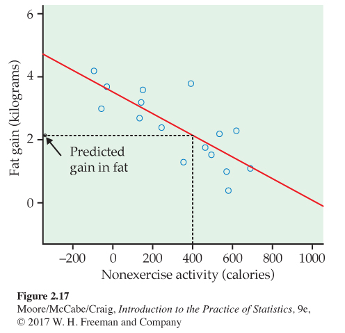
The figure shows that this line fits the data well. The slope b1 = −0.00344 tells us that fat gained goes down by 0.00344 kilogram for each added calorie of NEA increase.
The slope b1 of a line y = b0 + b1x is the average change in the response y as the explanatory variable x changes. The slope of a regression line is an important numerical description of the relationship between the two variables. For Example 2.20, the intercept, b0 = 3.505 kilograms. This value is the estimated fat gain if NEA does not change. When we substitute the value zero for the NEA increase, the regression equation gives 3.505 (the intercept) as the predicted value of the fat gain.
USE YOUR KNOWLEDGE
Question 2.61
2.61 Plot the line. Make a plot of the data in Example 2.19 and plot the line
fat gain = 4.505 − (0.00344 × NEA increase)
on your sketch. Explain why this line does not give a good fit to the data.
2.61 (a) Almost all the data points are below the line.
Prediction
We can use a regression line to predictprediction the response y for a specific value of the explanatory variable x. We can interpret the prediction as the average value of y corresponding to a collection of cases at the particular value of x or as our best guess at the value of y for an individual with the particular value of x.
EXAMPLE 2.21
Prediction for fat gain. Based on the linear pattern, we want to predict the fat gain for an individual whose NEA increases by 400 calories when she overeats. To use the fitted line to predict fat gain, go “up and over” on the graph in Figure 2.17. From 400 calories on the x axis, go up to the fitted line and over to the y axis. The graph shows that the predicted gain in fat is a bit more than 2 kilograms.
If we have the equation of the line, it is faster and more accurate to substitute x = 400 in the equation. The predicted fat gain is
fat gain = 3.505 − (0.00344 × 400) = 2.13 kilograms
The accuracy of predictions from a regression line depends on how much scatter about the line the data show. In Figure 2.17, fat gains for similar increases in NEA show a spread of 1 or 2 kilograms. The regression line summarizes the pattern but gives only roughly accurate predictions.
USE YOUR KNOWLEDGE
Question 2.62
2.62 Predict the fat gain. Use the regression equation in Example 2.20 to predict the fat gain for a person whose NEA increases by 250 calories.
EXAMPLE 2.22
Is this prediction reasonable? Can we predict the fat gain for someone whose nonexercise activity increases by 1500 calories when she overeats? We can certainly substitute 1500 calories into the equation of the line. The prediction is
fat gain = 3.505 − (0.00344 × 1500) = −1.66 kilograms
That is, we predict that this individual loses fat when she overeats. This prediction is not trustworthy. Look again at Figure 2.17. An NEA increase of 1500 calories is far outside the range of our data. We can’t say whether increases this large ever occur, or whether the relationship remains linear at such extreme values. Predicting fat gain when NEA increases by 1500 calories extrapolates the relationship beyond what the data show.
EXTRAPOLATION
Extrapolation is the use of a regression line for prediction far outside the range of values of the explanatory variable x used to obtain the line. Such predictions are often not accurate and should be avoided.
USE YOUR KNOWLEDGE
Question 2.63
2.63 Would you use the regression equation to predict? Consider the following values for NEA increase: −300, 300, 600, 800. For each, decide whether you would use the regression equation in Example 2.20 to predict fat gain or whether you would be concerned that the prediction would not be trustworthy because of extrapolation. Give reasons for your answers.
2.63 Predictions for 300 and 600 are trustworthy: interpolation. Predictions from − 300 and 800 are not trustworthy: extrapolation.
Least-squares regression
Different people might draw different lines by eye on a scatterplot. This is especially true when the points are widely scattered. We need a way to draw a regression line that doesn’t depend on our guess as to where the line should go. No line will pass exactly through all the points, but we want one that is as close as possible. We will use the line to predict y from x, so we want a line that is as close as possible to the points in the vertical direction. That’s because the prediction errors we make are errors in y, which is the vertical direction in the scatterplot.
The line in Figure 2.17 predicts 2.13 kilograms of fat gain for an increase in nonexercise activity of 400 calories. If the actual fat gain turns out to be 2.3 kilograms, the error is
error = observed gain − predicted gain
= 2.3 − 2.13 = 0.17 kilogram
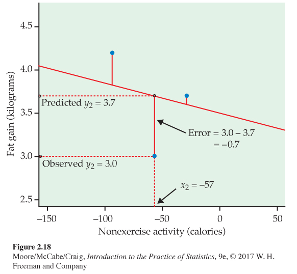
Errors are positive if the observed response lies above the line and negative if the response lies below the line. We want a regression line that makes these prediction errors as small as possible. Figure 2.18 illustrates the idea. For clarity, the plot shows only three of the points from Figure 2.17, along with the line, on an expanded scale. The line passes below two of the points and above one of them. The vertical distances of the data points from the line appear as vertical line segments. A “good” regression line makes these distances as small as possible. There are many ways to make “as small as possible” precise. The most common is the least-squares idea. The line in Figures 2.17 and 2.18 is, in fact, the least-squares regression line.
LEAST-SQUARES REGRESSION LINE
The least-squares regression line of y on x is the line that makes the sum of the squares of the vertical distances of the data points from the line as small as possible.
Here is the least-squares idea expressed as a mathematical problem. We represent n observations on two variables x and y as
(x1, y1), (x2, y2), . . ., (xn, yn)
If we draw a line y = b0 + b1x through the scatterplot of these observations, the line predicts the value of y corresponding to xi as ˆyi=b0 + b1xi. We write ˆy (read “y-hat”) in the equation of a regression line to emphasize that the line gives a predicted response ˆy for any x. The predicted response will usually not be exactly the same as the actually observed response y. The method of least squares chooses the line that makes the sum of the squares of these errors as small as possible. To find this line, we must find the values of the intercept b0 and the slope b1 that minimize
∑(error)2=∑(yi−b0−b1xi)2
for the given observations x1 and y1. For the NEA data, for example, we must find the b0 and b1 that minimize
(4.2−b0+94b1)2+(3.0−b0+57b1)2+⋯+(1.1−b0−690b1)2
These values are the intercept and slope of the least-squares line.
You will use software or a calculator with a regression function to find the equation of the least-squares regression line from data on x and y. Therefore, we will give the equation of the least-squares line in a form that helps our understanding but is not efficient for calculation.
EQUATION OF THE LEAST-SQUARES REGRESSION LINE
We have data on an explanatory variable x and a response variable y for n individuals. The means and standard deviations of the sample data are ˉx and sx for x and ˉy and sy for y, and the correlation between x and y is r. The equation of the least-squares regression line of y on x is
ˆy=b0 + b1x
with slope
b1=r sysx
and intercept
b0=ˉy − b1ˉx
EXAMPLE 2.23
Check the calculations. Verify from the data in Example 2.19 that the mean and standard deviation of the 16 increases in NEA are
ˉx=324.8 calories and sx=257.66 calories
The mean and standard deviation of the 16 fat gains are
ˉy=2.388 kg and sy=1.1389 kg
The correlation between fat gain and NEA increase is r = −0.7786. Therefore, the least-squares regression line of fat gain y on NEA increase x has slope
b1=r sysx=−0.7786 1.1389257.66
=−0.00344 kg per calorie
and intercept
b0=ˉy − b1ˉx
=2.388 − (−0.00344)(324.8)=3.505 kg
The equation of the least-squares line is
ˆy=3.505 − 0.00344x
![]()
When doing calculations like this by hand, you may need to carry extra decimal places in the preliminary calculations to get accurate values of the slope and intercept. Using software or a calculator with a regression function eliminates this worry.
Interpreting the regression line
The slope b1 = −0.00344 kilograms per calorie in Example 2.23 is the change in fat gain as NEA increases. The units “kilograms of fat gained per calorie of NEA” come from the units of y (kilograms) and x (calories). Although the correlation does not change when we change the units of measurement, the equation of the least-squares line does change. The slope in grams per calorie would be 1000 times as large as the slope in kilograms per calorie because there are 1000 grams in a kilogram. The small value of the slope, b1 = −0.00344, does not mean that the effect of increased NEA on fat gain is small—it just reflects the choice of kilograms as the unit for fat gain. The slope and intercept of the least-squares line depend on the units of measurement—you can’t conclude anything from their size.
![]()
EXAMPLE 2.24
Regression using software. Figure 2.19 displays the basic regression output for the nonexercise activity data from three statistical software packages. Other software produces very similar output. You can find the slope and intercept of the least-squares line, calculated to more decimal places than we need, in each output. The software also provides information that we do not yet need, including some that we trimmed from Figure 2.19.
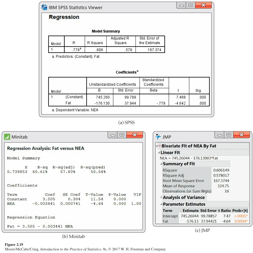
Part of the art of using software is to ignore the extra information that is almost always present. Look for the results that you need. Once you understand a statistical method, you can read output from almost any software.
Facts about least-squares regression
Regression is one of the most common statistical settings, and least squares is the most common method for fitting a regression line to data. Here are some facts about least-squares regression lines.
Fact 1. There is a close connection between correlation and the slope of the least-squares line. The slope is
b1=r sysx
This equation says that along the regression line, a change of one standard deviation in x corresponds to a change of r standard deviations in y. When the variables are perfectly correlated (r = 1 or r = −1), the change in the predicted response ˆy is the same (in standard deviation units) as the change in x. Otherwise, because −1 ≤ r ≤ 1, the change in ˆy is less than the change in x. As the correlation grows less strong, the prediction y moves less in response to changes in x. Note that if the correlation is zero, then the slope of the least-squares regression line will be zero.
Fact 2. The least-squares regression line always passes through the point (ˉx, ˉy) on the graph of y against x. So, the least-squares regression line of y on x is the line with slope rsy/sx that passes through the point (ˉx, ˉy). We can describe regression entirely in terms of the basic descriptive measures ˉx, sx, ˉy, sy, and r.
Fact 3. The distinction between explanatory and response variables is essential in regression. Least-squares regression looks at the distances of the data points from the line only in the y direction. If we reverse the roles of the two variables, we get a different least-squares regression line.
Correlation and regression
Least-squares regression looks at the distances of the data points from the line only in the y direction. So the two variables x and y play different roles in regression.
EXAMPLE 2.25
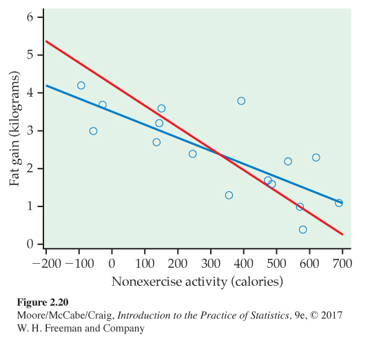
Fidgeting and fat gain. Figure 2.20 is a scatterplot of the fidgeting and fat gain data described in Example 2.19 (page 107). There is a negative linear relationship. The two lines on the plot are the two least-squares regression lines. The regression line using nonexercise activity to predict fat gain is blue. The regression line using fat gain to predict nonexercise activity is red. Regression of fat gain on nonexercise activity and regression of nonexercise activity on fat gain give different lines. In the regression setting, you must decide which variable is explanatory.
Even though the correlation r ignores the distinction between explanatory and response variables, there is a close connection between correlation and regression. We saw that the slope of the least-squares line involves r. Another connection between correlation and regression is even more important. In fact, the numerical value of r as a measure of the strength of a linear relationship is best interpreted by thinking about regression. Here is the fact we need.
r2 IN REGRESSION
The square of the correlation, r2, is the fraction of the variation in the values of y that is explained by the least-squares regression of y on x.
The correlation between NEA increase and fat gain for the 16 subjects in Example 2.19 (page 107) is r = −0.7786. Because r2 = 0.6062, the straight-line relationship between NEA and fat gain explains about 61% of the vertical scatter in fat gains in Figure 2.17 (page 109).
When you report a regression, give r2 as a measure of how successfully the regression explains the response. All three software outputs in Figure 2.19 include r2, either in decimal form or as a percent.
When you see a correlation, square it to get a better feel for the strength of the association. Perfect correlation (r = −1 or r = 1) means that the points lie exactly on a line. Then r2 = 1 and all the variation in one variable is accounted for by the linear relationship with the other variable. If r = −0.7 or r = 0.7, r2 = 0.49 and about half the variation is accounted for by the linear relationship. In the r2 scale, correlation ±0.7 is about halfway between 0 and ±1.
USE YOUR KNOWLEDGE
Question 2.64
2.64 What fraction of the variation is explained? Consider the following correlations: −0.9, −0.5, −0.2, 0, 0.2, 0.5, and 0.9. For each, give the fraction of the variation in y that is explained by the least-squares regression of y on x. Summarize what you have found from performing these calculations.
The use of r2 to describe the success of regression in explaining the response y is very common. It rests on the fact that there are two sources of variation in the responses y in a regression setting. Figure 2.17 (page 109) gives a rough visual picture of the two sources. The first reason for the variation in fat gains is that there is a relationship between fat gain y and increase in NEA x. As x increases from −94 to 690 calories among the 16 subjects, it pulls fat gain y with it along the regression line in the figure. The linear relationship explains this part of the variation in fat gains.
The fat gains do not lie exactly on the line, however, but are scattered above and below it. This is the second source of variation in y, and the regression line tells us nothing about how large it is. The dashed lines in Figure 2.17 show a rough average for y when we fix a value of x. We use r2 to measure variation along the line as a fraction of the total variation in the fat gains. In Figure 2.17, about 61% of the variation in fat gains among the 16 subjects is due to the straight-line relationship between y and x. The remaining 39% is vertical scatter in the observed responses remaining after the line has fixed the predicted responses.
Another view of r2
Here is a more specific interpretation of r2. The fat gains y in Figure 2.17 range from 0.4 to 4.2 kilograms. The variance of these responses, a measure of how variable they are, is
variance of observed values y = 1.297
Much of this variability is due to the fact that as x increases from −94 to 690 calories, it pulls y along with it. If the only variability in the observed responses were due to the straight-line dependence of fat gain on NEA, the observed gains would lie exactly on the regression line. That is, they would be the same as the predicted gains ˆy. We can compute the predicted gains by substituting the NEA values for each subject into the equation of the least-squares line. Their variance describes the variability in the predicted responses. The result is
variance of predicted values ˆy=0.786
This is what the variance would be if the responses fell exactly on the line; that is, if the linear relationship explained 100% of the observed variation in y. Because the responses don’t fall exactly on the line, the variance of the predicted values is smaller than the variance of the observed values. Here is the fact we need:
r2=variance of predicted valuesˆyvariance of observed valuesy=0.7861.297=0.606
This fact is always true. The squared correlation gives the variance that the responses would have if there were no scatter about the least-squares line as a fraction of the variance of the actual responses. This is the exact meaning of “fraction of variation explained” as an interpretation of r2.
These connections with correlation are special properties of least-squares regression. They are not true for other methods of fitting a line to data. One reason that least squares is the most common method for fitting a regression line to data is that it has many convenient special properties.