SECTION 2.4 EXERCISES
For Exercise 2.61, see page 109; for Exercise 2.62, see page 110; for Exercise 2.63, see page 111; and for Exercise 2.64, see page 116.
Question 2.65
2.65 Blueberries and anthocyanins. In Exercise 2.18 (page 97), you examined the relationship between Antho4 and Antho3, two anthocyanins found in blueberries. In Exercise 2.42 (page 105), you found the correlation between these two variables.
(a) Find the equation of the least-squares regression line for predicting Antho4 from Antho3.
(b) Make a scatterplot of the data with the fitted line.
(c) How well does the line fit the data? Explain your answer.
(d) Use the line to predict the value of Antho4 when Antho3 is equal to 1.5.
2.65 (a) ˆy = 0.34475 + 0.15185Antho3. (c) The line does not fit the data well. (d) ˆy = 0.572525.
Question 2.66
2.66 Fuel consumption. In Exercise 2.21 (page 97), you examined the relationship between CO2 emissions and highway fuel consumption for 527 vehicles that use regular fuel. In Exercise 2.44 (page 105), you found the correlation between these two variables.
(a) Find the equation of the least-squares regression line for predicting CO2 emissions from highway fuel consumption.
(b) Make a scatterplot of the data with the fitted line.
(c) How well does the line fit the data? Explain your answer.
(d) Use the line to predict the value of CO2 for vehicles that consume 8.0 liters per kilometer (L/km).
Question 2.67
2.67 Fuel consumption for different types of vehicles. In Exercise 2.23 (page 97), you examined the relationship between CO2 emissions and highway fuel consumption for 1067 vehicles. You used different plotting symbols for the four different types of fuel used by these vehicles: regular, premium, diesel, and ethanol.
(a) Find the least-squares equation for predicting CO2 emissions from highway fuel consumption for all 1067 vehicles.
(b) Make a scatterplot of the data with the fitted line.
(c) Based on what you learned from Example 2.23, do you think that a single least-squares regression line provides a good fit for all four types of vehicles? Explain your answer.
2.67 (a) ˆy = 56.75012 + 20.78205FuelConsHwy. (c) A single regression line would not be a good fit for the four types of vehicles, even though the correlations were all very close. There are several different lines that need to be accounted for.
Question 2.68
2.68 Bone strength. Exercise 2.24 (page 97), gives the bone strengths of the dominant and the nondominant arms for 15 men who were controls in a study.
(a) Plot the data. Use the bone strength in the nondominant arm as the explanatory variable and bone strength in the dominant arm as the response variable.
(b) The least-squares regression line for these data is
dominant = 2.74 + (0.936 × nondominant)
Add this line to your plot.
(c) Use the scatterplot (a graphical summary), with the least-squares line (a graphical display of a numerical summary) to write a short paragraph describing this relationship.
Question 2.69
2.69 Bone strength for baseball players. Refer to the previous exercise. Similar data for baseball players are given in Exercise 2.25 (page 98). Here is the equation of the least-squares line for the baseball players:
dominant = 0.886 + (1.373 × nondominant)
Answer parts (a) and (c) of the previous exercise for these data.
2.69 (c) There is a strong linear relationship. For each unit increase in nondominant, the dominant arm bone strength increases by 1.373.
Question 2.70
2.70 Predict the bone strength. Refer to Exercise 2.68. A young male who is not a baseball player has a bone strength of 16.0 cm4/1000 in his nondominant arm. Predict the bone strength in the dominant arm for this person.
Question 2.71
2.71 Predict the bone strength for a baseball player. Refer to Exercise 2.69. A young male who is a baseball player has a bone strength of 16.0 cm4/1000 in his nondominant arm. Predict the bone strength in the dominant arm for this person.
2.71 Predicted bone strength is 22.854 cm4/1000.
Question 2.72
2.72 Compare the predictions. Refer to the two previous exercises. You have predicted two dominant-arm bone strengths, one for a baseball player and one for a person who is not a baseball player. The nondominant bone strengths are both 16.0 cm4/1000.
(a) Compare the two predictions by computing the difference in means, baseball player minus control.
(b) Explain how the difference in the two predictions is an estimate of the effect of baseball throwing exercise on the strength of arm bones.
(c) For nondominant arm strengths of 12 cm4/1000 and 20 cm4/1000, repeat your predictions and take the differences. Make a table of the results of all three calculations (for 12, 16, and 20 cm4/1000).
(d) Write a short summary of the results of your calculations for the three different nondominant-arm strengths. Be sure to include an explanation of why the differences are not the same for the three nondominant-arm strengths.
Question 2.73
2.73 Least-squares regression for radioactive decay. Refer to Exercise 2.32 (page 99) for the data on radioactive decay of barium-137m. Here are the data:
| Time | 1 | 3 | 5 | 7 |
| Count | 578 | 317 | 203 | 118 |
(a) Using the least-squares regression equation
count = 602.8 − (74.7 × time)
find the predicted values for the counts.
(b) Compute the differences, observed count minus predicted count. How many of these are positive; how many are negative?
(c) Square and sum the differences that you found in part (b).
(d) Repeat the calculations that you performed in parts (a), (b), and (c) using the equation
count = 500 − (100 × time)
(e) In a short paragraph, explain the least-squares idea using the calculations that you performed in this exercise.
2.73 (a) − (c)
| Count = 602.8 − (74.7 × time) | ||||
|---|---|---|---|---|
| Time | Count | Predicted | Difference | Squared difference |
| 1 | 578 | 528.1 | 49.9 | 2490.01 |
| 3 | 317 | 378.7 | − 61.7 | 3806.89 |
| 5 | 203 | 229.3 | − 26.3 | 691.69 |
| 7 | 118 | 79.9 | 38.1 | 1451.61 |
(d)
| Count = 500 − (100 × time) | ||||
|---|---|---|---|---|
| Time | Count | Predicted | Difference | Squared difference |
| 1 | 578 | 400 | 178 | 31,684 |
| 3 | 317 | 200 | 117 | 13,689 |
| 5 | 203 | 0 | 203 | 41,209 |
| 7 | 118 | − 200 | 318 | 101,124 |
(e) The first line is a better description of the relationship.
Question 2.74
2.74 Least-squares regression for the log counts. Refer to Exercise 2.33 (page 99), where you analyzed the radioactive decay of barium-137m data using log counts. Here are the data:
| Time | 1 | 3 | 5 | 7 |
| Log count | 6.35957 | 5.75890 | 5.31321 | 4.77068 |
(a) Using the least-squares regression equation
log count = 6.593 − (0.2606 × time)
find the predicted values for the log counts.
(b) Compute the differences, observed count minus predicted count. How many of these are positive; how many are negative?
(c) Square and sum the differences that you found in part (b).
(d) Repeat the calculations that you performed in parts (a), (b), and (c) using the equation
log count = 7 − (0.2 × time)
(e) In a short paragraph, explain the least-squares idea using the calculations that you performed in this exercise.
Question 2.75
2.75 College students by state. How well does the population of a state predict the number of undergraduates? The National Center for Educational Statistics collects data for each of the 50 U.S. states that we can use to address this question.18
- Page 120
(a) Make a scatterplot with population on the x axis and number of undergraduates on the y axis.
(b) Describe the form, direction, and strength of the relationship. Are there any outliers?
(c) For the number of undergraduates, the mean is 302,136 and the standard deviation is 358,460, and for population, the mean is 5,955,551 and the standard deviation is 6,620,733. The correlation between the number of undergraduates and the population is 0.98367. Use this information to find the least-squares regression line. Show your work.
(d) Add the least-squares line to your scatterplot.
2.75 (b) The relationship is linear, positive and strong. There are several outliers. (c) ˆy = − 15057 + 0.05326x.
Question 2.76
2.76 College students by state without the four largest states. Refer to the previous exercise. Let’s eliminate the four largest states, which have populations greater than 15 million. Here are the numerical summaries: for number of undergraduate college students, the mean is 220,134 and the standard deviation is 165,270; for population, the mean is 4,367,448 and the standard deviation is 3,310,957. The correlation between the number of undergraduate college students and the population is 0.97081. Use this information to find the least-squares regression line. Show your work.
Question 2.77
2.77 Make predictions and compare. Refer to the two previous exercises. Consider a state with a population of 4 million (this value is approximately the median population for the 50 states).
(a) Using the least-squares regression equation for all 50 states, find the predicted number of undergraduate college students.
(b) Do the same using the least-squares regression equation for the 46 states with populations less than 15 million.
(c) Compare the predictions that you made in parts (a) and (b). Write a short summary of your results and conclusions. Pay particular attention to the effect of including the four states with the largest populations in the prediction equation for a median-sized state.
2.77 (a) ˆy = 197,993. (b) ˆy = 202,327. (c) The outliers didn’t change the prediction for the median-sized state.
Question 2.78
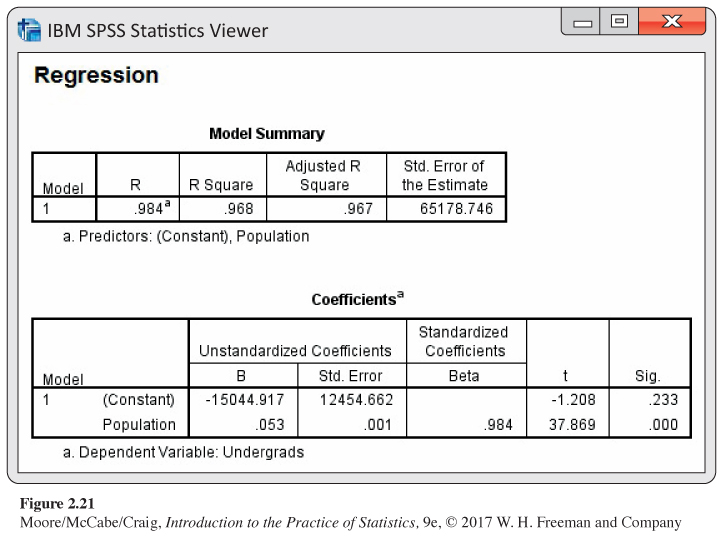
2.78 College students by state. Refer to Exercise 2.75, where you examined the relationship between the number of undergraduate college students and the populations for the 50 states. Figure 2.21 gives the output from a software package for the regression. Use this output to answer the following questions:
(a) What is the equation of the least-squares regression line?
(b) What is the value of r2?
(c) Interpret the value of r2.
(d) Does the software output tell you that the relationship is linear and not, for example, curved? Explain your answer.
Question 2.79
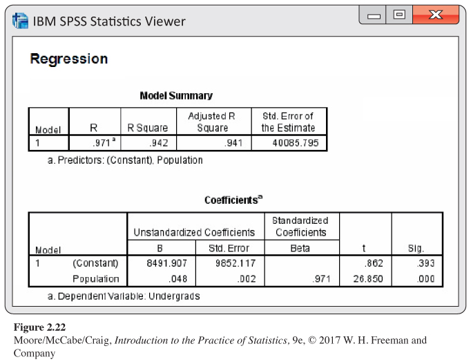
2.79 College students by state without the four largest states. Refer to Exercise 2.76, where you eliminated the four largest states that have populations greater than 15 million. Figure 2.22 gives software output for these data. Answer the questions in the previous exercise for the data set with the 46 states.
2.79 (a) ˆy = 8491.907 + 0.048x. (b) r2 = 0.942. (c) 94.2% of the variation in the number of undergraduates is accounted for by the population size. (d) The software does not report nature of the relationship.
Question 2.80
2.80 Data generated by software. The following 20 observations on Y and X were generated by a computer program.
| X | Y | X | Y |
|---|---|---|---|
| 22.06 | 34.38 | 17.75 | 27.07 |
| 19.88 | 30.38 | 19.96 | 31.17 |
| 18.83 | 26.13 | 17.87 | 27.74 |
| 22.09 | 31.85 | 20.20 | 30.01 |
| 17.19 | 26.77 | 20.65 | 29.61 |
| 20.72 | 29.00 | 20.32 | 31.78 |
| 18.10 | 28.92 | 21.37 | 32.93 |
| 18.01 | 26.30 | 17.31 | 30.29 |
| 18.69 | 29.49 | 23.50 | 28.57 |
| 18.05 | 31.36 | 22.02 | 29.80 |
(a) Make a scatterplot and describe the relationship between Y and X.
(b) Find the equation of the least-squares regression line and add the line to your plot.
(c) What percent of the variability in Y is explained by X?
(d) Summarize your analysis of these data in a short paragraph.
Question 2.81
2.81 Add an outlier. Refer to Exercise 2.80. Add an additional observation with y = 25 and x = 35 to the data set. Repeat the analysis that you performed in Exercise 2.80 and summarize your results, paying particular attention to the effect of this outlier.
2.81 (a) There is a weak positive linear relationship but with one extreme outlier. (b) ˆy = − 7.28789 + 1.89089x. (c) r2 = 0.7715. (d) Although the x variable accounts for 77.15% of the variation in y, there is a very high outlier for x, which pulls the regression line unnaturally, accounting for the jump in R-square.
Question 2.82
2.82 Add a different outlier. Refer to Exercise 2.80 and the previous exercise. Add an additional observation with y = 36 and x = 30 to the original data set.
(a) Repeat the analysis that you performed in Exercise 2.80 and summarize your results, paying particular attention to the effect of this outlier.
(b) In this exercise and in the previous one, you added an outlier to the original data set and reanalyzed the data. Write a short summary of the changes in correlations that can result from different kinds of outliers.
Question 2.83
2.83 Alcohol and calories in beer. Figure 2.12 (page 98) gives a scatterplot of calories versus percent alcohol in 159 brands of domestic beer.
(a) Find the equation of the least-squares regression line for these data.
(b) Find the value of r2 and interpret it in the regression context.
Page 122Table : TABLE 2.1 Four Data Sets for Exploring Correlation and RegressionData Set A x 10 8 13 9 11 14 6 4 12 7 5 y 8.04 6.95 7.58 8.81 8.33 9.96 7.24 4.26 10.84 4.82 5.68 Data Set B x 10 8 13 9 11 14 6 4 12 7 5 y 9.14 8.14 8.74 8.77 9.26 8.10 6.13 3.10 9.13 7.26 4.74 Data Set C x 10 8 13 9 11 14 6 4 12 7 5 y 7.46 6.77 12.74 7.11 7.81 8.84 6.08 5.39 8.15 6.42 5.73 Data Set D x 8 8 8 8 8 8 8 8 8 8 19 y 6.58 5.76 7.71 8.84 8.47 7.04 5.25 5.56 7.91 6.89 12.50 (c) Write a short report on the relationship between calories and percent alcohol in beer. Include graphical and numerical summaries for each variable separately as well as graphical and numerical summaries for the relationship in your report.
2.83 (a) ˆy = 6.41895 + 28.34687x. (b) r2 = 0.8193. (c) The relationship between calories and percent alcohol is linear, positive, and strong; however, there does seem to be one low outlier, O’Douls, with a very low alcohol content.
Question 2.84
2.84 Alcohol and calories in beer revisited. Refer to the previous exercise. The data that you used includes an outlier.
(a) Remove the outlier and answer parts (a), (b), and (c) for the new set of data.
(d) Write a short paragraph about the possible effects of outliers on a least-squares regression line and the value of r2, using this example to illustrate your ideas.
Question 2.85
2.85 Always plot your data! Table 2.1 presents four sets of data prepared by the statistician Frank Anscombe to illustrate the dangers of calculating without first plotting the data.19
(a) Without making scatterplots, find the correlation and the least-squares regression line for all four data sets. What do you notice? Use the regression line to predict y for x = 10.
(b) Make a scatterplot for each of the data sets and add the regression line to each plot.
(c) In which of the four cases would you be willing to use the regression line to describe the dependence of y on x? Explain your answer in each case.
2.85 (a) The correlations and regression lines for all four data sets are essentially the same: r = 0.82 and ˆy = 3 + 0.5x. For x = 10, ˆy = 8. (c) Only for data set A should regression be used.
Question 2.86
2.86 Progress in math scores. Every few years, the National Assessment of Educational Progress asks a national sample of eighth-graders to perform the same math tasks. The goal is to get an honest picture of progress in math. Here are the last few national mean scores, on a scale of 0 to 500:20
| Year | 1990 | 1992 | 1996 | 2000 | 2003 | 2005 | 2008 | 2011 | 2013 |
| Score | 263 | 268 | 272 | 273 | 278 | 279 | 281 | 283 | 285 |
(a) Make a time plot of the mean scores, by hand. This is just a scatterplot of score against year. There is a slow linear increasing trend.
(b) Find the regression line of mean score on time step-by-step. First calculate the mean and standard deviation of each variable and their correlation (use a calculator with these functions). Then find the equation of the least-squares line from these. Draw the line on your scatterplot. What percent of the year-to-year variation in scores is explained by the linear trend?
(c) Now use software or the regression function on your calculator to verify your regression line.
Question 2.87
2.87 The regression equation. The equation of a least-squares regression line is y = 15 − 2x.
(a) What is the value of y for x = 4?
(b) If x increases by one unit, what is the corresponding change in y?
(c) What is the intercept for this equation?
2.87 (a) y = 7. (b) For each unit increase in x, y decreases by 2. (c) 15.
Question 2.88
2.88 Metabolic rate and lean body mass. Compute the mean and the standard deviation of the metabolic rates and lean body masses in Exercise 2.37 (page 100) and the correlation between these two variables. Use these values to find the slope of the regression line of metabolic rate on lean body mass. Also find the slope of the regression line of lean body mass on metabolic rate. What are the units for each of the two slopes?
Question 2.89
![]() 2.89 Use an applet for progress in math scores. Go to the Two-Variable Statistical Calculator. Enter the data for the progress in math scores from Exercise 2.86 using the “User-entered data” option in the “Data” tab. Explore the data by clicking the other tabs in the applet. Using only the only the results provided by the applet, write a short report summarizing the analysis of these data.
2.89 Use an applet for progress in math scores. Go to the Two-Variable Statistical Calculator. Enter the data for the progress in math scores from Exercise 2.86 using the “User-entered data” option in the “Data” tab. Explore the data by clicking the other tabs in the applet. Using only the only the results provided by the applet, write a short report summarizing the analysis of these data.
2.89 ˆy=0.896x−1517.935. r = 0.982. We can conclude that NAEP scores are steadily increasing about 0.896 point per year.
Question 2.90
![]() 2.90 A property of the least-squares regression line. Use the equation for the least-squares regression line to show that this line always passes through the point (ˉx, ˉy).
2.90 A property of the least-squares regression line. Use the equation for the least-squares regression line to show that this line always passes through the point (ˉx, ˉy).
Question 2.91
2.91 Class attendance and grades. A study of class attendance and grades among first-year students at a state university showed that, in general, students who missed a higher percent of their classes earned lower grades. Class attendance explained 16% of the variation in grade index among the students. What is the numerical value of the correlation between percent of classes attended and grade index?
2.91 r = 0.4.