4.3 4.3 Random Variables
When you complete this section, you will be able to:
• Describe the probability distribution of a discrete random variable.
• Use a probability histogram to provide a graphical description of the probability distribution of a discrete random variable.
• Use the distribution of a discrete random variable to calculate probabilities of events.
• Find probabilities of events for the uniform and normal distributions.
Sample spaces need not consist of numbers. When we toss a coin four times, we can record the outcome as a string of heads and tails, such as HTTH. In statistics, however, we are most often interested in numerical outcomes such as the count of heads in the four tosses. It is convenient to use a shorthand notation: Let X be the number of heads. If our outcome is HTTH, then X = 2. If the next outcome is TTTH, the value of X changes to X = 1. The possible values of X are 0, 1, 2, 3, and 4. Tossing a coin four times will give X one of these possible values. Tossing four more times will give X another and probably different value. We call X a random variable because its values vary when the coin tossing is repeated.
RANDOM VARIABLE
A random variable is a variable whose value is a numerical outcome of a random process.
In our earlier coin-tossing example, the process is the tossing of a coin four times. The random variable is the number of heads in the four tosses.
We usually denote random variables by capital letters near the end of the alphabet, such as X or Y. Of course, the random variables of greatest interest to us are outcomes such as the mean ˉx of a random sample, for which we will keep the familiar notation.9 As we progress from general rules of probability toward statistical inference, we will concentrate on random variables.
When a random variable X describes a random process, the sample space S just lists the possible values of the random variable. We usually do not mention S separately. There remains the second part of any probability model, the assignment of probabilities to events. There are two main ways of assigning probabilities to the values of a random variable. The two types of probability models that result will dominate our application of probability to statistical inference.
Discrete random variables
We have learned several rules of probability, but only one method of assigning probabilities: state the probabilities of the individual outcomes and assign probabilities to events by summing over the outcomes. The outcome probabilities must be between 0 and 1 and have sum 1. When the outcomes are numerical, they are values of a random variable. We will now attach a name to random variables having probability assigned in this way.10
DISCRETE RANDOM VARIABLE
A discrete random variable X has possible values that can be given in an ordered list. The probability distribution of X lists the values and their probabilities:
| Value of X | x1 | x2 | x3 | . . . |
| Probability | p1 | p2 | p3 | . . . |
The probabilities pi must satisfy two requirements:
1. Every probability pi is a number between 0 and 1.
2. p1 + p2 + · · · = 1.
Find the probability of any event by adding the probabilities pi of the particular values xi that make up the event.
In most discrete random variable situations that we will study, the number of possible values is a finite number, k. For example, in our example on the number of heads in four tosses of a coin, there are k = 5 possible values: 0, 1, 2, 3, and 4.
There are, however, settings in which the number of possible values can be infinite. Think about tossing a fair coin until you get a head. The number of possible tosses is any positive integer.
EXAMPLE 4.22
Grade distributions. A liberal arts college posts the grade distributions for its courses. In a recent semester, students in one section of English 130 received 32% A’s, 42% B’s, 19% C’s, 3% D’s, and 4% F’s. Choose an English 130 student at random. To “choose at random” means to give every student the same chance to be chosen. The student’s grade on a five-point scale (with A = 4) is a random variable X.
The value of X changes when we repeatedly choose students at random, but it is always one of 0, 1, 2, 3, or 4. Here is the distribution of X:
| Value of X | 0 | 1 | 2 | 3 | 4 |
| Probability | 0.04 | 0.03 | 0.19 | 0.42 | 0.32 |
The probability that the student got a B or better is the sum of the probabilities of an A and a B. In the language of random variables,
P(X ≥ 3) = P(X = 3) + P(X = 4)
= 0.42 + 0.32 = 0.74
USE YOUR KNOWLEDGE
Question 4.42
4.42 Will the course satisfy the requirement? Refer to Example 4.22. Suppose that a grade of D or F in English 130 does not satisfy a requirement for a major in linguistics. What is the probability that a randomly selected student will not satisfy this requirement?
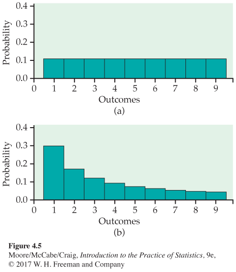
We can use histograms to show probability distributions as well as distributions of data. Figure 4.5 displays probability histogramsprobability histogram that compare the probability model for equally likely random digits (Example 4.15, page 227) with the model given by Benford’s law (Example 4.12, page 226). The height of each bar shows the probability of the outcome at its base. Because the heights are probabilities, they add to 1. As usual, all the bars in a histogram have the same width. So the areas also display the assignment of probability to outcomes. Think of these histograms as idealized pictures of the results of very many trials. The histograms make it easy to quickly compare the two distributions.
EXAMPLE 4.23
Number of heads in four tosses of a coin. What is the probability distribution of the discrete random variable X that counts the number of heads in four tosses of a coin? We can derive this distribution if we make two reasonable assumptions:
• The coin is balanced, so it is fair and each toss is equally likely to give H or T.
• The coin has no memory, so tosses are independent.
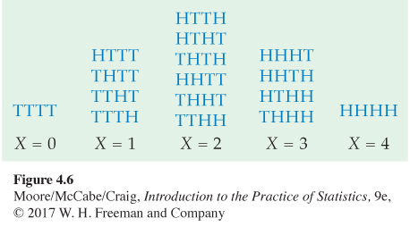
The outcome of four tosses is a sequence of heads and tails such as HTTH. There are 16 possible outcomes in all. Figure 4.6 lists these outcomes along with the value of X for each outcome. The multiplication rule for independent events tells us that, for example,
P(HTTH)=12×12×12×12=116
Each of the 16 possible outcomes similarly has probability 1/16. That is, these outcomes are equally likely.
The number of heads X has possible values 0, 1, 2, 3, and 4. These values are not equally likely. As Figure 4.6 shows, there is only one way that X = 0 can occur: namely, when the outcome is TTTT. So
P(X=0)=116=0.0625
The event {X = 2} can occur in six different ways, so that
P(X=2)=countofwaysX=2canoccur16=616=0.375
We can find the probability of each value of X from Figure 4.6 in the same way. Here is the result:
| Value of X | 0 | 1 | 2 | 3 | 4 |
| Probability | 0.0625 | 0.25 | 0.375 | 0.25 | 0.0625 |
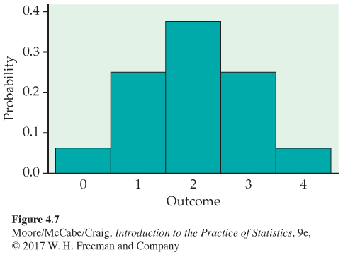
Figure 4.7 is a probability histogram for the distribution in Example 4.23. The probability distribution is exactly symmetric. The probabilities (bar heights) are idealizations of the proportions after very many tosses of four coins. The actual distribution of proportions observed would be nearly symmetric but is unlikely to be exactly symmetric.
EXAMPLE 4.24
Probability of at least three heads. Any event involving the number of heads observed can be expressed in terms of X, and its probability can be found from the distribution of X. For example, the probability of tossing at least three heads is
P(X ≥ 3) = 0.25 + 0.0625 = 0.3125
The probability of at least one head is most simply found by use of the complement rule:
P(X≥1)=1-P(X=0)=1-0.0625=0.9375
Recall that tossing a coin n times is similar to choosing an SRS of size n from a large population and asking a Yes or No question. We will extend the results of Example 4.23 when we return to sampling distributions in the next chapter.
USE YOUR KNOWLEDGE
Question 4.43
4.43 Two tosses of a fair coin. Find the probability distribution for the number of heads that appear in two tosses of a fair coin.
4.43 Possible values: 0, 1, 2. Probabilities: 1/4, 1/2, 1/4.
Continuous random variables
When we use the table of random digits to select a digit between 0 and 9, the result is a discrete random variable. The probability model assigns probability 1/10 to each of the 10 possible outcomes. Suppose that we want to choose a number at random between 0 and 1, allowing any number between 0 and 1 as the outcome. Software random number generators will do this.
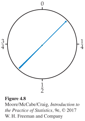
You can visualize such a random number by thinking of a spinner (Figure 4.8) that turns freely on its axis and slowly comes to a stop. The pointer can come to rest anywhere on a circle that is marked from 0 to 1. The sample space is now an entire interval of numbers:
S = {all numbers x such that 0 ≤ x ≤ 1}
density curve, p. 51
How can we assign probabilities to events such as {0.3 ≤ x ≤ 0.7}? As in the case of selecting a random digit, we would like all possible outcomes to be equally likely. But we cannot assign probabilities to each individual value of x and then sum because there are too many possible values. Instead, we use a new way of assigning probabilities directly to events—as areas under a density curve. Any density curve has area exactly 1 underneath it, corresponding to total probability 1.
EXAMPLE 4.25
Uniform random numbers. The random number generator will spread its output uniformly across the entire interval from 0 to 1 as we allow it to generate a long sequence of numbers. The results of many trials are represented by the density curve of a uniform distributionuniform distribution.
This density curve appears in red in Figure 4.9. It has height 1 over the interval from 0 to 1, and height 0 everywhere else. The area under the density curve is 1: the area of a square with base 1 and height 1. The probability of any event is the area under the density curve and above the event in question.
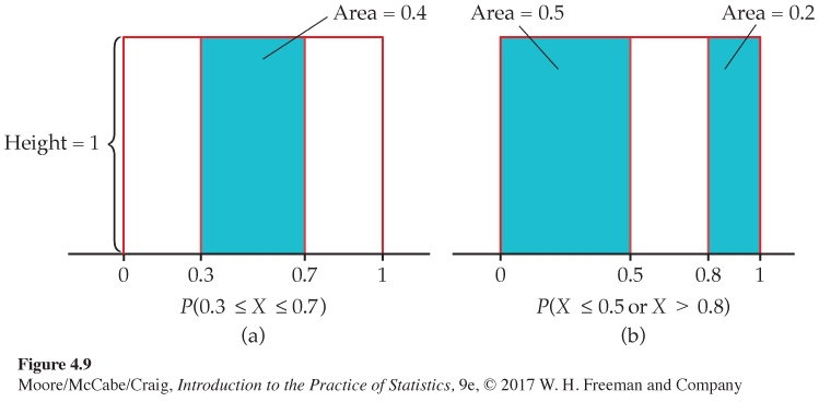
As Figure 4.9(a) illustrates, the probability that the random number generator produces a number X between 0.3 and 0.7 is
P(0.3 ≤ X ≤ 0.7) = 0.4
because the area under the density curve and above the interval from 0.3 to 0.7 is 0.4. The height of the density curve is 1, and the area of a rectangle is the product of height and length, so the probability of any interval of outcomes is just the length of the interval.
Similarly,
P(X ≤ 0.5) = 0.5
P(X > 0.8) = 0.2
P(X ≤ 0.5 or X > 0.8) = 0.7
Notice that the last event consists of two nonoverlapping intervals, so the total area above the event is found by adding two areas, as illustrated by Figure 4.9(b). This assignment of probabilities obeys all of our rules for probability.
USE YOUR KNOWLEDGE
Question 4.44
4.44 Find the probability. For the uniform distribution described in Example 4.25, find the probability that X is between 0.3 and 0.9.
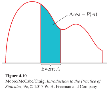
Probability as area under a density curve is a second important way of assigning probabilities to events. Figure 4.10 illustrates this idea in general form. We call X in Example 4.25 a continuous random variable because its values are not isolated numbers but an entire interval of numbers.
CONTINUOUS RANDOM VARIABLE
A continuous random variable X takes all values in an interval of numbers. The probability distribution of X is described by a density curve. The probability of any event is the area under the density curve and above the values of X that make up the event.
The probability model for a continuous random variable assigns probabilities to intervals of outcomes rather than to individual outcomes. In fact, all continuous probability distributions assign probability 0 to every individual outcome. Only intervals of values have positive probability. To see that this is true, consider a specific outcome such as P(X = 0.8) in the context of Example 4.25. The probability of any interval is the same as its length. The point 0.8 has no length, so its probability is 0.
Although this fact may seem odd, it makes intuitive, as well as mathematical, sense. The random number generator produces a number between 0.79 and 0.81 with probability 0.02. An outcome between 0.799 and 0.801 has probability 0.002. A result between 0.799999 and 0.800001 has probability 0.000002. You see that as we approach 0.8, the probability gets closer to 0.
To be consistent, the probability of an outcome exactly equal to 0.8 must be 0. Because there is no probability exactly at X = 0.8, the two events {X > 0.8} and {X ≥ 0.8} have the same probability. We can ignore the distinction between > and ≥ when finding probabilities for continuous (but not discrete) random variables.
![]()
Normal distributions as probability distributions
Normal distributions, p. 56
The density curves that are most familiar to us are the Normal curves. Because any density curve describes an assignment of probabilities, Normal distributions are probability distributions. Recall that N(μ, σ) is our shorthand for the Normal distribution having mean μ and standard deviation σ. In the language of random variables, if X has the N(μ, σ) distribution, then the standardized variable
Z=X−μσ
is a standard Normal random variable having the distribution N(0,1).
EXAMPLE 4.26
Texting while driving. Texting while driving can be dangerous, but young people want to remain connected. Suppose that 26% of teen drivers text while driving. If we take a sample of 500 teen drivers, what percent would we expect to say that they text while driving?11
The proportion p = 0.26 is a number that describes the population of teen drivers. The proportion ˆp of the sample who say that they text while driving is used to estimate p. The proportion ˆp is a random variable because repeating the SRS would give a different sample of 500 teen drivers and a different value of ˆp.
We will see in the next chapter that in this setting, with teen drivers answering honestly, ˆp has approximately the N(0.26, 0.0196) distribution. The mean 0.26 of this distribution is the same as the population proportion because ˆp is an unbiased estimate of p. The standard deviation is controlled mainly by the size of the sample.
What is the probability that the survey result differs from the truth about the population by no more than 3 percentage points? We can use what we learned about Normal distribution calculations to answer this question. Because p = 0.26, the survey misses by no more than 3 percentage points if the sample proportion is between 0.23 and 0.29.
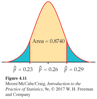
Figure 4.11 shows this probability as an area under a Normal density curve. You can find it by software or by standardizing and using Table A. From Table A,
P(0.23≤ˆp≤0.29)=P(0.23-0.260.0196≤ˆp-0.260.0196≤0.29-0.260.0196)=P(-1.53≤Z≤1.53)=0.9370-0.0630=0.8740
About 87% of the time, the sample ˆp will be within 3 percentage points of the proportion p.
We began this chapter with a general discussion of the idea of probability and the properties of probability models. Two very useful specific types of probability models are distributions of discrete and continuous random variables. In our study of statistics, we will employ only these two types of probability models.